creel survey, fisheries, design-based inference, R, tidycreel, Quarto
5.1 Purpose
Recreational fishing is one of the most widely practiced outdoor activities in North America, yet the fisheries that support it are among the least precisely monitored. Unlike commercial fisheries, where landings are recorded at processing facilities and catch limits are enforced at the dock, recreational harvest is spread across thousands of access points, compressed into short seasonal windows, and produced by anglers who usually are not required to report what they caught. The result is a system in which substantial fishing pressure and harvest can accumulate out of sight, and the first indication that a population is in trouble may arrive years after the damage has been done (Pope et al. in press).
Creel surveys are built to close that gap. By sending trained clerks into the field to count anglers and conduct structured interviews, fisheries agencies collect the raw material needed to estimate total effort, total catch, and angler behavior across a defined fishery and time period. Done well, a creel survey converts a partially observed, spatially distributed recreational fishery into a set of statistically defensible estimates that can be compared across years, presented to regulatory bodies, and used to justify changes in harvest regulations or stocking programs.
The economic stakes are real. The U.S. Fish and Wildlife Service estimates that recreational anglers spend tens of billions of dollars annually on equipment, travel, and license fees. In many states, sport fishing license revenue is the primary funding mechanism for fisheries conservation programs. The fish populations that support this activity are a public trust resource, and fisheries agencies are obligated — legally in some jurisdictions — to manage that resource using the best available information about harvest and effort. Creel surveys remain one of the standard ways agencies generate that information.
The basic method has been around for decades. Roving creel surveys were described in the North American literature by the 1950s, and the statistical foundations for estimation from instantaneous counts were formalized by Pollock et al. (1994) and colleagues at a symposium that produced a synthesis still widely cited today. What has changed is the computational environment. Modern creel datasets involve thousands of records, multiple strata, incomplete trips, species-level catch matrices, and the expectation that estimates will be accompanied by defensible variance estimates. Doing that work in spreadsheets — as many agencies still do — is error-prone, difficult to audit, and nearly impossible to replicate. This book is about how to do it reproducibly in R with the tidycreel package.
This chapter covers:
why recreational fisheries are harder to monitor than commercial ones, and what that means for survey design;
what creel surveys actually measure and the five core estimands;
how field records become fishery-wide inferences;
what reproducibility means in the creel survey context and why it matters;
how creel estimates connect to management decisions; and
a first look at what creel data look like, using Harlan Reservoir as a running example.
How this book is organized
This book is organized around the estimation workflow, not around individual concepts. Each chapter takes the output of the previous chapter as its input and produces output that feeds into the next. That structure mirrors what a practitioner actually does when working a real creel dataset from scratch.
Part I: Foundations (Chapters 1–3 plus Quick Start) lays the statistical foundation. Chapter 2 defines estimands formally, introduces notation, and describes the reporting domains that bound creel inference. Chapter 3 develops the design-based estimator, derives the variance formula, and works through a stratified effort estimate end to end. If you want the definitions first, start with Section 6.2; if you want the sampling logic, go to Section 5.5. The Quick Start chapter that closes Part I runs the entire estimation pipeline on Harlan data in a single session, front to back, before the formal treatment begins.
Part II: Survey Designs covers the four field methods in common use — access-point, roving, aerial and camera-assisted, and stratified designs — and closes with pre-survey planning (sample size, power analysis, schedule generation using creel_power() and generate_schedule()) and a chapter on bias and failure modes. This part is where design decisions are made; the estimation chapters that follow assume those decisions are already locked.
Part III: From Field to R bridges the gap between field collection and analysis. One chapter covers instrument design, interview protocols, and schedule validation using creel_schema() and validate_creel_schedule(). The other introduces tidycreel.connect, the companion package for reading creel data from CSV, SQL Server, and REST API backends into the linked-table structure that the rest of the book assumes.
Part IV: Data Structures and Validation (Chapters 9–11) covers the four-table data model, the creel_design object, and the cleaning steps — outlier flagging, species standardization, incomplete-trip review — that change estimates before analysis begins.
Part V: Estimation and Reporting (Chapters 12–16 plus three specialty chapters) introduces the core tidycreel estimation functions: estimate_effort(), estimate_total_harvest(), estimate_catch_rate(), and their release and biological counterparts. Additional chapters cover length and biomass estimation, uncertainty diagnostics and power analysis, full-season reporting, and multi-year trend detection with compare_designs() and weighted linear regression.
Part VI: Case Studies applies all methods to Cedar Lake, a roving creel survey on a warmwater reservoir, demonstrating the full pipeline from raw data to a management-ready report for a fishery that differs structurally from the Harlan access-point example used throughout the book.
5.2 Recreational fisheries as partially observed systems
Consider what a fisheries manager actually knows about recreational harvest on a 5,000-hectare reservoir on a given day. An unknown number of anglers are on the water, arriving and departing at irregular intervals. They fish from boats, from shore, from kayaks. They target different species with different gear. Some keep fish; most do not. Some will round, forget, or hedge a detail or two. By evening, everyone has gone home, and the day survives only in the notes collected by whoever happened to be in the field.
That is a partially observed system. The full population of fishing activity is never visible at once. The manager can observe only what a sampling design captures. Every inference about total effort, catch, or harvest is therefore an extrapolation from a sample — an estimate with uncertainty, not a count.
Misestimating recreational harvest has real consequences. Pope et al. (in press) notes that recreational harvest drives population dynamics of many socially, economically, and ecologically important fish species, and poorly quantified harvest has contributed to the collapse of important fisheries. Accurate, well-characterized estimates are not a scientific luxury; they are the information base for regulatory decisions that determine whether a fishery remains viable.
The target population and the sampling frame
Statistical inference requires a clearly defined target population — the set of all units about which the analyst wants to make statements — and a sampling frame — the operational list or procedure from which the sample is actually drawn. In creel surveys, the target population is all fishing activity at a waterbody during a defined time period. The sampling frame is the set of days, time periods, and access points from which the field crew draws its schedule.
The gap between the target population and the sampling frame is one of the most important concepts in creel design. A survey that samples only boat ramp access points excludes bank fishing. A survey that samples only from April through September excludes fall fishing. Estimates computed from that survey describe the sampled portion of the fishery, not the full fishery — unless the sampled portion is demonstrably the whole. This sounds obvious, but it is frequently obscured in creel reports that do not state explicitly what the frame was.
Temporal heterogeneity
Participation in recreational fishing varies dramatically across temporal scales. At the annual scale, most freshwater fisheries in the northern United States have a pronounced seasonal pattern: effort peaks in May and June, drops sharply through midsummer, and rises again in fall before the season closes. At the weekly scale, weekend effort is consistently two to four times higher than weekday effort on most reservoir fisheries, reflecting the working schedules of the angler population. At the daily scale, effort is concentrated in morning and late-afternoon hours on hot summer days, while cool spring and fall conditions spread effort more evenly across the day.
All of these patterns create a fundamental sampling challenge. A survey that samples uniform fractions of weekdays and weekends does not represent the fishery proportionally by effort. A survey that sends crews out only in the morning misses the late-afternoon concentrated fishing that may produce a large fraction of summer harvest. A stratified design addresses these problems by defining strata — typically combinations of day type and season — within which conditions are internally more homogeneous than across the entire survey period. Sampling and estimation then proceed within strata, and stratum totals are summed to produce the seasonal estimate. The strata must be defined before the sample is drawn, not after.
Spatial heterogeneity
Reservoir fisheries are also spatially heterogeneous. Different sections of a large reservoir attract different types of fishing activity. The tailwater below a dam may concentrate bank anglers fishing for catfish. Shallow coves support bass fishing from small boats. Open main-lake habitat is favored by walleye trollers. Each section may have different catch rates, different gear, and different angler demographics. A creel design that monitors only a subset of access points — because they are convenient — produces estimates biased toward the activity at those points.
On large systems, spatial stratification is necessary. The reservoir is divided into sections with defined access points, and each section is sampled independently. On small systems where one or two access points handle most of the traffic, spatial stratification may be unnecessary. The design decision depends on the spatial structure of the fishery, which is one reason that pilots or initial reconnaissance surveys are valuable before committing to a multi-year design.
Angler heterogeneity
Beyond time and space, anglers themselves are heterogeneous. Experienced anglers catch more fish per hour. Tournament anglers travel farther and concentrate effort differently than casual anglers. Charter boat clients fish longer trips and have higher catch rates than wade anglers. Gear type — baitcasting for bass, jigging for walleye, bottom rigs for catfish — is correlated with both catch rate and species composition. None of these sources of angler heterogeneity can be eliminated from the sampling problem; they can only be described through the interview data collected alongside the counts.
This is one reason that the interview component of a creel survey collects more than just the raw catch count. Information about trip duration, party size, angler type, target species, and gear allows the analyst to understand whether changes in estimated catch rates across years reflect changes in fish abundance or changes in the angler population. A declining CPUE trend that coincides with a shift toward less experienced anglers is a very different management signal than one that occurs against a stable angler population.
5.3 Types of creel surveys
Not all creel surveys use the same field methods. The two broadest categories are access point surveys and roving surveys, and the choice between them has consequences for both logistics and estimation.
Access point surveys
In an access point survey, the field clerk stations at one or more defined points — typically boat ramps, parking areas, or bank fishing sites — and interviews anglers as they complete their trips and exit the fishery. Effort is estimated separately, using counts taken from a vantage point or a roving route that covers the waterbody. The separation of count operations from interview operations is a practical advantage: the clerk stationed at the ramp can conduct thorough interviews while a second observer completes the count route, and both operations can proceed simultaneously on large waters.
Access point surveys have a potential bias: they intercept only anglers who exit through the monitored access point. Anglers who use unmonitored access — unmarked trails, private land, or canoe carries — are not counted, not interviewed, and not represented in the estimate. On waterbodies with complex or unofficial access, this exclusion can be substantial. Pilot surveys that map all access points and estimate their usage fractions are essential before committing to an access-point design.
The statistical framework for access point estimation is well developed. Under certain conditions, the probability that an angler is intercepted at the access point during the clerk’s presence can be estimated, and the inverse of that probability serves as the expansion factor for observed catch. The tidycreel function estimate_effort() implements this framework with support for stratification by day type, period, and section.
Roving surveys
In a roving survey, the field clerk travels a defined route — typically by boat on reservoir surveys — stopping to count and interview anglers encountered along the way. The route is designed to cover the survey area in a single pass, and the timing of the pass is randomized within a defined window. This design has the advantage of covering the full waterbody and not relying on a defined exit point, making it well suited to waters with dispersed or informal access.
The estimation challenge in roving surveys is that anglers encountered mid-trip are at different stages of their fishing day. The clerk records what the angler has caught so far, but the angler has not yet completed the trip. Inferring total daily catch requires additional information: either a follow-up interview at trip completion (the “bus route” design described in Pollock et al. (1994)) or a statistical model of the expected additional catch given time already fished. Both approaches are implemented in tidycreel and discussed in Chapter 5.
Hybrid and specialized designs
Many agencies use hybrid designs that combine elements of access point and roving surveys, or that add passive monitoring components. A common hybrid assigns access point clerks during peak morning traffic and sends a roving clerk along the count route during off-peak hours. Camera systems at boat ramps reduce labor costs for the count component while preserving interview coverage. Aerial surveys are used on large systems — primarily for effort estimation — and can be integrated with ground-based interview programs.
The choice of design depends on waterbody characteristics, agency resources, and the precision requirements imposed by management questions. Chapter 6 provides a framework for evaluating design options through power analysis before the first field day.
5.4 What creel surveys do
A creel survey combines two field operations that are conducted on each sampled day: counts and interviews.
Counts
Counts are instantaneous observations of the number of anglers present at a waterbody or access site at a specific moment in time. On small, visually open waterbodies, a clerk can complete a true instantaneous count by observing the entire system at once. On larger systems, the clerk travels between vantage points quickly enough that no anglers arrive or depart during the traversal — what Pope et al. (in press) describes as a functionally instantaneous count. The count is recorded with a timestamp and the clerk’s location; it is not an interview and does not involve talking to anglers.
Counts do not estimate effort by themselves. They become an effort estimate only when the analyst combines them with the length of the fishing day and an estimate of how long trips last on average. Under the usual assumptions, the count is treated as a snapshot of angler density, then expanded to angler-hours through the design-based estimator in Chapter 3.
Counts are typically conducted at multiple points during a sampled day, within randomized “count periods.” Randomizing when within a day the counts occur — rather than always counting at 8 AM or at noon — is a design requirement, not a nicety. Systematic count times introduce bias if effort is not constant across the day, which it never is in practice.
Some survey programs augment or replace roving counts with passive monitoring: cameras at boat ramps that record angler departures, automated fish counters, or aerial observation on large water bodies. The tidycreel package provides estimation functions for both roving and camera-based count designs. The inferential logic is similar; the data format and estimation equation differ.
Interviews
Interviews are structured conversations with anglers, typically conducted when they complete a trip. The clerk records how long the angler fished, how many anglers were in the party, what they targeted, what they caught, what they kept, and sometimes whether they have any fish available for measurement. The interview happens at an access point, a boat ramp, or along a shoreline — on-site, not by mail or phone later.
This temporal proximity to the fishing activity is the defining advantage of creel surveys over mail or telephone recall methods: anglers interviewed as they leave the water usually remember the trip more accurately than anglers contacted weeks later (Pope et al. in press). Recall error grows quickly as the delay increases, which is why same-day intercept interviews are usually much more reliable than retrospective reports.
The biological information collected during interviews — species composition, lengths, weights, tissue samples — also provides secondary confirmation of what was caught and can support stock assessment directly. Length frequency data from creel interviews, for example, can be used alongside mark-recapture data in integrated assessment models. This secondary use of creel data is often overlooked in agency planning but can substantially increase the information return per dollar spent in the field.
One logistical challenge is that some trips are incomplete at the time of intercept — the angler has not yet finished fishing and cannot report total catch. Incomplete trip records require special treatment in estimation, either through imputation of expected additional catch, through weighting by probability of completion, or through exclusion with appropriate design adjustments. Chapter 5 covers incomplete trip handling in detail.
How counts and interviews connect
The two streams of information — counts and interviews — combine to produce population-level estimates. Counts scale the interview data up to the fishery as a whole: the interview provides a catch rate (fish per angler-hour), and the count-derived effort estimate provides the total angler-hours, so the product yields total catch. Neither stream alone produces an estimate; both are necessary.
This means that errors in either stream propagate into every downstream estimate. A systematic undercounting of bank anglers (because the clerk’s route does not include a hidden access point) inflates the apparent catch rate even if interviews are accurate, because the denominator (angler-hours) is underestimated. A systematic bias in reported trip duration — anglers round down to avoid looking like they were “fishing all day” — deflates the catch rate used in the effort multiplier. Understanding the potential sources of bias in both streams is part of what makes creel survey design a specialized discipline rather than a generic sampling problem.
The five core estimands
Every creel survey addresses some subset of five estimands. Understanding each is essential because they have different denominators, different field collection requirements, and different risks of misinterpretation.
Effort (E) is the total fishing time expended by all anglers at a waterbody or access site during a defined time period, usually expressed in angler-hours or angler-trips. Effort is the foundational estimand: it appears in the denominator of catch rates and scales all per-trip or per-hour counts up to seasonal totals. Underestimating effort produces inflated catch-rate estimates even when the interview data are accurate. Effort is estimated from the count stream, not from interviews.
A simple representation: if \hat{U}_t is the estimated number of angler-hours on day t, and there are T days in the season, then total seasonal effort is:
\hat{E} = \sum_{t=1}^{T} \hat{U}_t
In practice, \hat{U}_t is estimated from instantaneous count data using the relationship between mean count and mean trip duration, stratified by day type. Chapter 3 derives this estimator in full.
Total catch (C) is the number of fish encountered by all anglers during a time period, regardless of whether those fish were retained or released. Total catch includes fish that were caught and kept (harvest) and fish that were caught and returned (release). Reporting total catch is important when the management question is about fish removed from the population through any mechanism — including catch-and-release mortality. Total catch is estimated by multiplying the catch rate per angler-hour (from interviews) by the total effort estimate (from counts):
\hat{C} = \hat{r} \cdot \hat{E}
where \hat{r} is the estimated catch rate (fish per angler-hour) from the interview sample.
Total harvest (H) is the subset of total catch consisting of fish retained by anglers. Harvest drives exploitation and is the key input to harvest-based stock assessments. Harvest regulation — bag limits, size limits, season closures — acts on harvest, so harvest estimates are the most direct link between creel surveys and management action. In many fisheries, harvest is the primary estimand and everything else is secondary.
Total release (R) is the subset of total catch consisting of fish returned to the water. In catch-and-release fisheries, total release is the dominant catch component. Release estimates matter for assessing release mortality, which can be substantial in some gear-and-species combinations, and for reconstructing the full interaction between anglers and the fish population. The accounting identity C = H + R provides a useful cross-check: estimated total catch should equal estimated harvest plus estimated release within sampling error.
Catch rate (CPUE) is the ratio of catch to effort: fish per angler-hour, fish per trip, or some similarly scaled unit. Catch rate is the most widely used diagnostic for changes in fish availability over time. A declining CPUE trend suggests either that the fish population has declined or that angler behavior has changed in ways that reduce catch efficiency. Interpreting CPUE trends requires understanding which of these mechanisms is operating, which is why CPUE estimates from creel surveys are always most useful when accompanied by information about angler behavior, gear, and target species.
These five estimands are not interchangeable. The same field records support different calculations depending on which estimand is the target. A design adequate for estimating seasonal total harvest may not be adequate for estimating month-specific catch rates. Writing down the target estimand — and the reporting domain over which it applies — before designing the survey is the most important step in creel survey planning.
TipSetting estimands before sampling
Estimands should be written down before the first clerk enters the field. A survey designed to estimate seasonal total walleye harvest may not have sufficient sample size to estimate weekly walleye catch rates, even from the same field records. Discovering mid-season that the question has changed often means starting the design over.
A worked miniature example
Consider a simple two-day example to make the relationships among estimands concrete. Suppose on a Monday a clerk counts 12 boat anglers at 10 AM. Average trip duration from Monday’s interviews is 4.2 hours, and the mean catch rate (all species combined) from those interviews is 0.8 fish per angler-hour, of which 60% were harvested.
From the count: \hat{U}_{\text{Mon}} = 12 \times 4.2 = 50.4 angler-hours (this simplification assumes the count at 10 AM represents average daily density; Chapter 3 formalizes the conversion).
From the interviews:
Estimated total catch (Monday): \hat{C}_{\text{Mon}} = 0.8 \times 50.4 = 40.3 fish
Estimated total harvest: \hat{H}_{\text{Mon}} = 0.60 \times 40.3 = 24.2 fish
Estimated total release: \hat{R}_{\text{Mon}} = 0.40 \times 40.3 = 16.1 fish
Catch rate (CPUE): 0.8 fish per angler-hour (directly from interviews)
Now suppose the same waterbody has 65 eligible weekdays in the season, of which 15 were sampled, and the mean estimated daily effort across those 15 days is 47 angler-hours. The seasonal weekday effort estimate is \hat{E}_{\text{WD}} = 65 \times 47 = 3{,}055 angler-hours. Multiplied by the mean weekday catch rate, this yields the seasonal weekday catch estimate. Repeating for the weekend stratum and summing the two stratum estimates yields the seasonal total.
This miniature example captures the full logical chain: count \rightarrow effort \rightarrow total catch \rightarrow harvest/release split. The core functions in tidycreel each implement some portion of this chain on real stratified datasets. The formalism of Chapter 3 extends this logic to cover stratification, variance estimation, and incomplete trip correction.
5.5 From field records to fishery-wide inference
A single day’s field records — a count sheet and a stack of interview forms — do not add up to a season estimate. That leap from sampled day to seasonal total is the inferential core of creel estimation, and it is where most errors in creel analysis are made.
The basic estimator
The basic structure is straightforward. Within each stratum s, there are N_s eligible days, of which n_s are sampled. On each sampled day, the analyst computes the day-specific effort \hat{U}_{s,t} and catch \hat{C}_{s,t}. The stratum-level total is:
\hat{T}_s = N_s \cdot \bar{U}_s
where \bar{U}_s = \frac{1}{n_s}\sum_{t=1}^{n_s}\hat{U}_{s,t} is the mean estimated daily effort within stratum s. Total seasonal effort is then:
This is a ratio estimator: within each sampled day, the count data yield an effort estimate, and those estimates are averaged and scaled by the total number of eligible days. The variance of the seasonal estimate accumulates across strata:
where s_s^2 is the within-stratum variance of daily effort estimates across sampled days. This finite-population correction — the term \left(1 - \frac{n_s}{N_s}\right) — is often negligible when the sampling fraction is small but can substantially reduce estimated variance when many days in a stratum are sampled.
Why stratification matters
The variance formula above makes clear why stratification reduces uncertainty. Within a stratum of homogeneous days, s_s^2 is small because similar conditions produce similar daily effort. Across a stratum that mixes high-effort summer weekends and low-effort November weekdays, s_s^2 is large. Stratifying the frame into internally homogeneous groups — typically by day type and season — reduces the within-stratum variance in each stratum, which directly reduces the total estimated variance.
The practical consequence: a survey with 40 sampled days spread across two well-chosen strata (weekdays and weekends) will have a substantially smaller confidence interval than a survey with 40 sampled days drawn uniformly from the season. Stratification is not free — it requires knowing the stratum boundaries before sampling — but it pays for itself in precision.
Precision targets and what “good” looks like
How much precision is enough? There is no universal answer, but practical guidance from the creel literature suggests that a coefficient of variation (CV = standard error / estimate) below 20–25% on the seasonal total is generally sufficient for harvest regulation decisions (Pollock et al. 1994). CVs below 10% are achievable on intensively sampled fisheries but require substantially more field days and are rarely necessary for routine management monitoring.
The relevant question is not “how precise can we get?” but “how precise do we need to be to support the management decision at hand?” A harvest estimate used to trigger a regulation review does not need the same precision as one used to parameterize a stock assessment model. Writing down the precision requirement before designing the survey is the creel equivalent of a power analysis: it translates an abstract statistical goal into a concrete sample size.
The pre-survey planning chapter in Part II develops the full power analysis framework using creel_power(), which accepts a hypothesized CV target and returns the number of sampled days needed to achieve it under a range of variance assumptions. Running this calculation before the first field day — not after — is the single most effective way to avoid underpowered surveys.
The role of auxiliary data
Some creel programs augment the probabilistic estimate with auxiliary data that can reduce variance or correct for known biases. Angler license sales provide an external estimate of participation that can serve as a benchmark for effort estimates: if the creel survey implies 40,000 angler-days but license records suggest far fewer active anglers in the fishery, the discrepancy warrants investigation. Electronic fish finders, trail cameras, and automatic vehicle counters have all been piloted as low-cost effort monitoring supplements that can reduce reliance on labor-intensive creel counts.
These auxiliary data sources do not replace the probabilistic creel survey but they can improve precision through ratio estimation or post-stratification. The statistical machinery for combining creel estimates with auxiliary information is similar to small-area estimation methods used in human demography. tidycreel does not yet implement full auxiliary-data integration, but Chapter 16 discusses the conceptual framework and points to survey package functionality that can be adapted for this purpose.
Design requirements for valid inference
What makes the estimator above more than bookkeeping is the design requirement. The estimator is unbiased only if:
the sampled days were drawn by probability sampling from the frame of all eligible days;
the strata used for estimation match the strata used for sampling;
the count times within each sampled day were randomized within the shift; and
each count is genuinely instantaneous (or functionally so).
Violating any of these conditions introduces bias. An access point count taken at the most convenient time of morning — say, 8:00 AM every day — is not a random instantaneous count. It reflects 8:00 AM conditions, which may differ systematically from mid-day or late-afternoon conditions on hot summer days when anglers avoid the heat. An estimate computed for a stratum that was not defined before sampling (for example, computing a “tournament weekend” estimate after the fact) cannot be weighted correctly because tournament days were not sampled as a separate stratum.
The sampling design is what authorizes the inferential leap from field records to population totals. Without a design, the field records are observations. With a design, they are evidence for a specific claim about the fishery during a specific period.
Important
The scope of inference is bounded by the sampling frame. A creel survey covering public boat ramp access from April to October produces estimates for public boat ramp access from April to October. It does not produce estimates for the whole year, for private access, or for species not targeted by the interviewed anglers. Expanding the inference beyond the frame is one of the most common errors in creel reporting.
5.6 Why reproducibility matters
Creel projects typically involve multiple people across multiple years. Field crews change. Database schemas evolve. The analyst who computed last year’s estimate may not be the one computing this year’s. In this environment, analyses that live in undocumented spreadsheets or ad hoc scripts become impossible to check, difficult to rerun when data are corrected, and impossible to compare reliably to prior years.
Reproducibility in the creel context means three things specifically:
The source data are traceable. Every observation in the analysis can be linked back to a field record. If a suspicious catch rate turns up in the data, the analyst should be able to identify which interview it came from, check it against the raw field form, and decide whether to flag or remove it. This traceability is not possible if the cleaning steps are undocumented or if data exist only in summarized form.
The analytical decisions are explicit. Every filtering rule, every stratum definition, every missing-data treatment is written down in code that runs and produces the same output each time. The rule “if trip duration was not recorded, impute from the mean” must be a line of code, not an informal judgment applied differently in different years.
The estimate can be rerun. When source records are corrected after a preliminary report — a transcription error fixed, a late interview added — the entire analysis should be re-executable from the corrected data without manual adjustment. That matters for agencies that issue preliminary season summaries and later revise them with finalized data.
These three properties are also what make creel estimates auditable in regulatory and legal contexts. When a proposed regulation change is based on creel data, the agency may need to defend the estimate to the public, to a legislative body, or to a peer reviewer. An estimate produced by a reproducible workflow can be defended step by step. An estimate produced by an undocumented chain of spreadsheet operations cannot.
What reproducibility looks like in R
A reproducible creel workflow starts with raw data from source files, applies documented transformations in sequence, and writes estimates to output files or tables. The key constraint is that every step must be code — no manual adjustments in Excel between the raw data and the final estimate.
That is the pattern used throughout this book. Each chapter introduces functions that operate on tidy data frames, produce tidy outputs, and chain together without undocumented intermediate steps.
tidycreel is designed around reproducibility. Every estimation function returns not just the point estimate but the data used to produce it, the variance, and the stratum-level components. Every function takes data frames as inputs and returns data frames as outputs, so each step in the analytical chain is auditable and re-runnable.
5.7 Common sources of error in creel estimation
Understanding where estimates go wrong is as important as understanding how they are computed correctly. The following errors appear repeatedly in the creel literature and in agency-level analyses.
Frame errors
A frame error occurs when the operational sampling frame does not cover the intended target population. The most common version is access-point exclusion: if the survey covers only the main boat ramp but a significant fraction of bank anglers enter via a public park half a mile away, those anglers are systematically excluded from counts, interviews, and estimates. The resulting estimates describe only the portion of the fishery accessed through the surveyed route.
Frame errors are insidious because they do not produce obvious warning signs in the data. The estimates look internally consistent; variance estimates may be small; confidence intervals may be narrow. The bias is visible only if an external check — a vehicle count at the unmonitored access, a tagged-fish return rate inconsistent with the harvest estimate — reveals a discrepancy.
The best protection against frame errors is a deliberate frame definition at the design stage: a physical map of all access points, an estimate of usage fractions for each, and a decision to either include all access or explicitly scope the inference to monitored access only.
Count-time bias
Count-time bias arises when instantaneous counts are systematically taken at times that do not represent the full distribution of angling effort across the day. On hot summer days, angling effort peaks in early morning and again in late afternoon; a survey that always counts at 10 AM captures an intermediate effort level that may underrepresent both peaks. If the count is intended to represent average daily density, it should be taken at a randomly selected time within the survey period.
This bias is straightforward to avoid — randomize count times within each shift during the design phase — but easy to neglect under field pressure. When field crews are short-staffed, the temptation is to take the count “when it’s convenient,” which typically means at arrival in the morning. Over a season, this produces systematically biased effort estimates whose direction and magnitude depend on the shape of the daily effort curve.
Incomplete trip inflation
Incomplete trips — anglers who have not yet finished fishing at the time of the interview — present a different problem. If incomplete trips are treated the same as complete trips in the estimation, catch rates are underestimated (because the angler has only reported partial catch) and the bias grows with mean trip duration. An angler halfway through a four-hour trip reports half the expected catch, contributing a catch rate that is approximately half the true completed-trip rate.
Several methods exist for handling incomplete trips: removing them and reweighting the remaining interviews, imputing the expected additional catch from a model of trip-length distributions, or using the “bus route” double-sampling design in which incomplete trips are re-interviewed at the end of the day. Each approach has different assumptions and different variance properties. tidycreel implements all three and Chapter 5 compares their performance on the Harlan dataset.
Stratum collapsing
When sample sizes within strata are small, the temptation is to collapse adjacent strata to stabilize variance estimates. Collapsing weekday and weekend strata because “there were only three sampled weekends this month” is a common workaround — but it destroys the design-based property of the estimator. If weekend effort is systematically higher than weekday effort (as Figure 5.2 shows for Harlan), pooling the two produces a biased estimate because the pooled mean is dominated by the more numerous sampled weekdays.
The correct response to small sample sizes is not stratum collapsing but power analysis at the design stage. If three weekends per month is insufficient to estimate weekend effort with adequate precision, the design needs more weekend sample days — not a post-hoc fix that discards the stratification structure.
Reviewer asymmetry
One subtler error arises not in the field or in estimation but in review and reporting. Creel estimates are presented to managers, legislative committees, and the public as point estimates — often without variance or confidence intervals. The estimate “12,400 walleye harvested” communicates precision it may not possess. If the 95% confidence interval on that estimate is 7,000–18,000, the management implications of being at the lower bound versus the upper bound are very different.
A commitment to reproducible workflows makes it natural to report uncertainty alongside estimates, because the variance is computed and stored in the same output object as the point estimate. When the variance has to be separately computed or recalled from memory, it tends to get omitted.
5.8 The management decision chain
Creel estimates do not exist for their own sake. They exist to inform management decisions. Understanding what those decisions are clarifies what level of precision is actually needed from the survey.
Harvest regulation
The most direct connection is to harvest regulation. Bag limits, size limits, and season dates are set based on assessments of whether current harvest levels are sustainable for the target fish population. An annual harvest estimate is the numerator in the exploitation rate; combined with a population abundance estimate, it tells the manager what fraction of the population anglers are removing each year. Sustainable harvest rates vary by species, population size, and productivity, but in many sport fisheries, exploitation rates above 30–40 percent are associated with population decline. A creel survey that can resolve annual harvest to within ±20 percent relative standard error is usually precise enough to detect regulation-triggering changes over a three- to five-year baseline.
Size limits, in particular, require length frequency data from creel surveys. A minimum length limit is only effective if the catch includes a meaningful proportion of fish near the limit. If angler-reported catch suggests that nearly all harvested walleye are already above 38 cm in a fishery with a 38 cm minimum, the limit is not the binding constraint and other regulatory tools may be more effective. Creel-derived length frequencies — collected during interviews — provide this diagnostic without requiring additional sampling programs.
Stocking programs
The second connection is to stocking programs. In put-and-take fisheries — where hatchery fish are stocked and expected to be harvested within one season — creel estimates of total harvest and harvest rate tell managers whether the stocking program is achieving its intended angler opportunity. If 10,000 rainbow trout are stocked and creel data suggest 7,000 were harvested, the program delivered 70 percent utilization. If the harvest estimate is 2,000, something went wrong: either stocking mortality was high, fish moved out of the survey area, or catch-and-release rates were much higher than expected (Harmon et al. 2018).
In put-and-grow fisheries — where hatchery fish are stocked at a small size and expected to grow for one or more seasons before harvest — creel surveys track the transition from stocked cohort to harvestable population. Annual length distributions in creel data, combined with stocking records, can identify whether the cohort is recruiting to the legal size limit on schedule.
Trend monitoring
The third connection is to trend monitoring. Most agencies run creel surveys not just for a single estimate but for a time series. Year-over-year changes in effort, harvest, and catch rates are the empirical basis for detecting changes in angler behavior and fish populations. This makes consistency across years particularly important. A change in sampling design, a change in strata definitions, or a change in how incomplete trips are handled can produce an apparent trend that is actually an artifact of the analytical method. Reproducible code and explicit documentation of design changes allow analysts to identify and communicate such artifacts.
A declining CPUE trend that triggers a regulation change should be robust to reasonable variation in analytical assumptions. When the same data produce very different trend estimates depending on how incomplete trips are handled, the trend itself is uncertain — and that uncertainty should be communicated alongside the point estimate.
Population assessment
The fourth connection is to population assessment. Creel surveys supply harvest estimates to stock assessment models. If the harvest estimate is biased, the assessment is biased regardless of how sophisticated the population model is. Creel estimation error propagates through every downstream analysis that uses it.
This coupling matters for survey design decisions. A stock assessment that requires harvest estimates with ±15 percent CV to produce stable recruitment estimates imposes a minimum precision requirement on the creel survey. Working backward from required assessment precision to required creel sample size — before any field work begins — is an underused but highly practical application of creel power analysis. The creel_power() function in tidycreel supports exactly this calculation.
5.9 A first look at creel data
Before going further, it is useful to see what creel data actually look like. This book uses Harlan Reservoir as a running example: a synthetic reservoir dataset with the structure, variance components, and species composition typical of a Nebraska plains reservoir fishery. The Harlan dataset consists of four linked tables representing a single survey season (April–October 2022).
# A tibble: 6 × 4
  interview_id species         catch_type n_fish
         <int> <chr>           <chr>       <int>
1            1 White Bass      released       11
2            1 White Bass      harvested      32
3            1 Yellow Perch    released        1
4            1 Walleye         released        0
5            4 White Bass      harvested       9
6            4 Freshwater Drum released        3
Before any analysis proceeds, validate_creel_data() confirms the tables are internally consistent — correct column types, no impossible values, no missing identifiers. This one call is the first step in every reproducible creel workflow. Chapter 9 covers the full validation battery.
── Creel Data Validation ───────────────────────────────────────────────────────
63 pass | 0 warn | 0 fail
── Table: counts ──
✔ reservoir
✔ type: class: character
✔ na_rate: 0 / 236 NA (0%)
✔ empty_strings: none
✔ date
✔ type: class: Date
✔ na_rate: 0 / 236 NA (0%)
✔ date_range: all within 1970-01-01 - 2100-12-31
✔ day_type
✔ type: class: character
✔ na_rate: 0 / 236 NA (0%)
✔ empty_strings: none
✔ period
✔ type: class: numeric
✔ na_rate: 0 / 236 NA (0%)
✔ negative_values: none
✔ section
✔ type: class: character
✔ na_rate: 0 / 236 NA (0%)
✔ empty_strings: none
✔ count_time
✔ type: class: character
✔ na_rate: 0 / 236 NA (0%)
✔ empty_strings: none
✔ bank_anglers
✔ type: class: integer
✔ na_rate: 0 / 236 NA (0%)
✔ negative_values: none
✔ angler_boats
✔ type: class: integer
✔ na_rate: 0 / 236 NA (0%)
✔ negative_values: none
✔ boat_anglers
✔ type: class: integer
✔ na_rate: 0 / 236 NA (0%)
✔ negative_values: none
── Table: interviews ──
✔ reservoir
✔ type: class: character
✔ na_rate: 0 / 600 NA (0%)
✔ empty_strings: none
✔ date
✔ type: class: Date
✔ na_rate: 0 / 600 NA (0%)
✔ date_range: all within 1970-01-01 - 2100-12-31
✔ day_type
✔ type: class: character
✔ na_rate: 0 / 600 NA (0%)
✔ empty_strings: none
✔ period
✔ type: class: numeric
✔ na_rate: 0 / 600 NA (0%)
✔ negative_values: none
✔ section
✔ type: class: character
✔ na_rate: 0 / 600 NA (0%)
✔ empty_strings: none
✔ interview_id
✔ type: class: integer
✔ na_rate: 0 / 600 NA (0%)
✔ negative_values: none
✔ party_id
✔ type: class: character
✔ na_rate: 0 / 600 NA (0%)
✔ empty_strings: none
✔ n_anglers
✔ type: class: numeric
✔ na_rate: 0 / 600 NA (0%)
✔ negative_values: none
✔ angler_type
✔ type: class: character
✔ na_rate: 0 / 600 NA (0%)
✔ empty_strings: none
✔ angler_method
✔ type: class: character
✔ na_rate: 0 / 600 NA (0%)
✔ empty_strings: none
✔ hours_fished
✔ type: class: numeric
✔ na_rate: 0 / 600 NA (0%)
✔ negative_values: none
✔ trip_status
✔ type: class: character
✔ na_rate: 0 / 600 NA (0%)
✔ empty_strings: none
The schedule table has one row per calendar day in the survey season, recording the day type (weekday or weekend) and whether that day was sampled. The counts table has one row per instantaneous count observation, linked to a day and period. The interviews table has one row per angler party per sampled day, recording trip characteristics and fishing effort. The catch table records the species composition of each party’s catch — one row per species per party per catch type (harvested or released), linked back to the interview record by interview_id.
This structure — four linked tables, not one wide spreadsheet — is the organizing principle of every chapter that follows. Understanding why these streams stay separate until the estimation step is the conceptual foundation of creel analysis in tidycreel. It is also the reason creel databases built from wide spreadsheets are difficult to analyze correctly: the joins required at estimation time are not obvious from a flat record, and the denominator for catch-rate calculations lives in a different table than the numerator.
Note
The Harlan Reservoir dataset is synthetic. Counts, catch rates, and species composition are drawn from distributions calibrated to typical Nebraska reservoir creel surveys, but they do not represent any specific real waterbody or agency dataset. Chapter 17 revisits the methods using a real published dataset.
The four-table data hierarchy
The four tables in the Harlan dataset represent four distinct levels of resolution in the creel data hierarchy:
harlan_schedule     one row per calendar day (211 rows)
  └── harlan_counts     one row per instantaneous count (236 rows)
  └── harlan_interviews one row per angler party per sampled day (600 rows)
        └── harlan_catch    one row per species per party per catch type (987 rows)
This hierarchy is not arbitrary — it reflects the logical structure of the estimation pipeline. The schedule defines which days were eligible and which were sampled; it is the denominator for the expansion from sample to population. The counts are taken on sampled days and provide the raw data for effort estimation. The interviews are also conducted on sampled days and provide catch rates. The catch records are at the finest resolution, disaggregated by species and catch type (harvested vs. released) within each interview.
The hierarchy means that joins must be performed in a specific order and that the appropriate denominator for each calculation lives at a specific level. Total walleye harvest, for example, is computed by: summing n_fish in harlan_catch where species == "Walleye" and catch_type == "harvested", grouping by interview_id; joining those party-level harvest totals back to harlan_interviews to get party size and hours fished; computing the catch rate per angler-hour; then multiplying by the effort estimate from harlan_counts and harlan_schedule. None of these steps can be short-circuited by collapsing the tables prematurely.
A wide flat table — where each row represents one interview and columns include species-specific catch fields — makes this pipeline harder, not easier. The long format forces the analyst to make the grouping logic explicit and prevents the quiet omission of species not encountered by a given party (which appear as absence records in the long format but simply as missing columns in a wide format). Throughout this book, all creel data are kept in the long four-table structure until the estimation step explicitly requires a join.
The sampling schedule
How many days were sampled, and how were they distributed across the season?
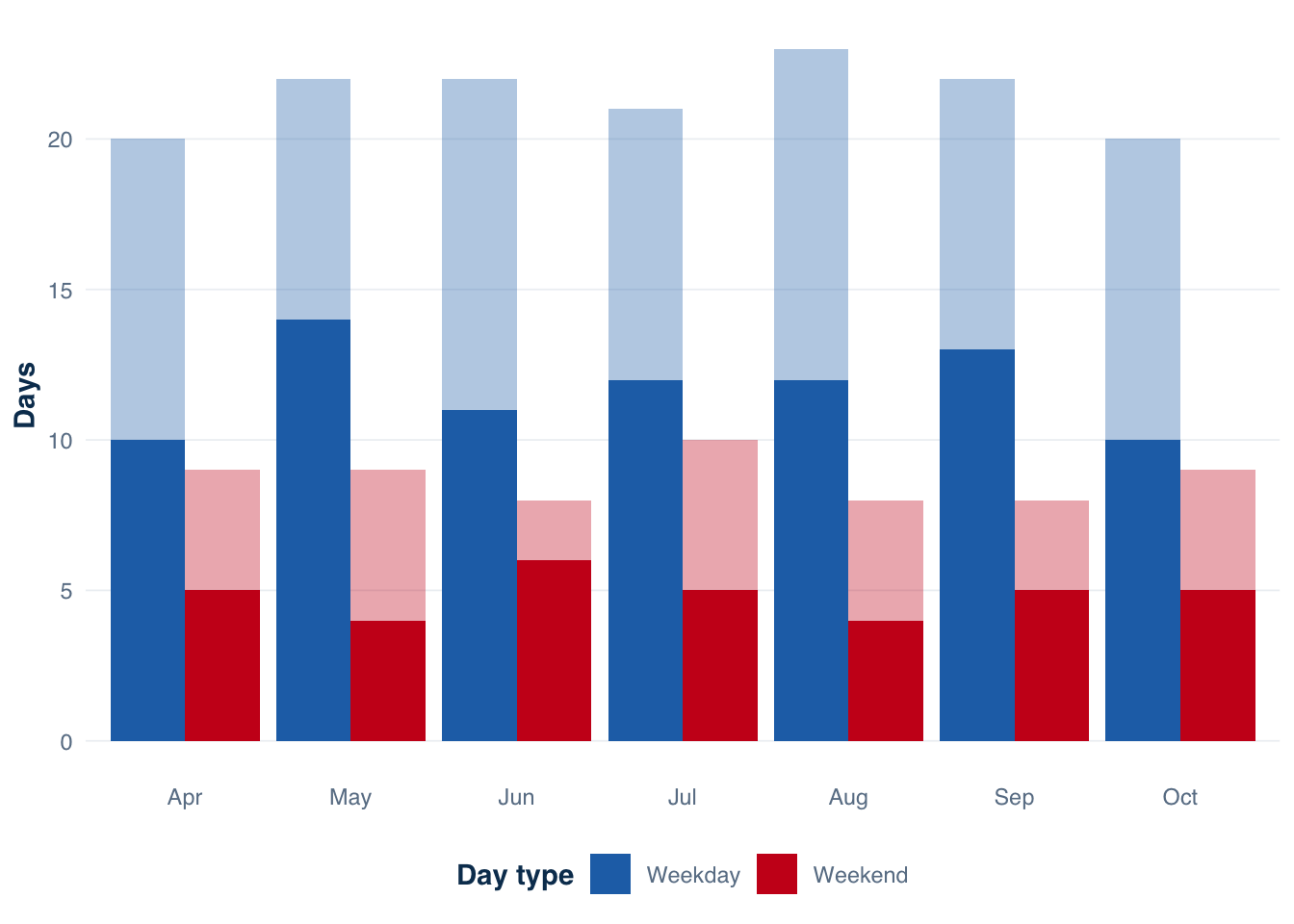
Figure 5.1: Sampled days at Harlan Reservoir by month and day type. Bars show the number of sampled days (shaded) out of all eligible days (total bar height) in each month-day-type stratum.
Figure 5.1 shows the sampling schedule across the seven-month season. Several features are immediately apparent. First, there are far more weekdays than weekend days in every month — a structural feature of the calendar that is not a design choice but must be accounted for in estimation. A stratum-weighted estimator down-weights weekday observations relative to the more-numerous weekend days only if strata are defined by day type before sampling. Second, the number of sampled days per month is roughly constant across the season, which is consistent with a proportional allocation design. Whether proportional allocation or optimal allocation (which would oversample high-variance months) is more appropriate depends on the pattern of within-month variance in effort — a topic taken up in Chapter 6.
Daily effort distribution
What does the distribution of effort look like across sampled days?
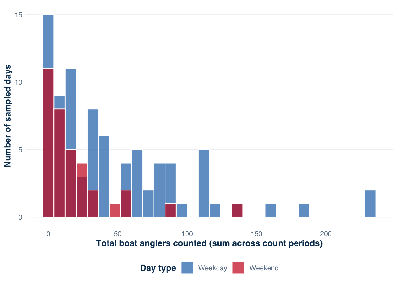
Figure 5.2: Distribution of total boat-angler counts per sampled day at Harlan Reservoir, by day type. Each observation is the sum of boat anglers recorded across all count periods on a given day. Weekend counts are shifted substantially higher than weekday counts, confirming the temporal heterogeneity that motivates day-type stratification.
Figure 5.2 shows the distribution of summed boat-angler counts per sampled day, split by day type. The weekend distribution is shifted substantially to the right of the weekday distribution — visual confirmation of the temporal heterogeneity discussed in the previous section. This difference in effort levels is the primary justification for day-type stratification: if weekday and weekend observations were pooled in a single stratum, the between-day variance would be inflated by the systematic difference between day types, increasing the width of the confidence interval on the seasonal effort estimate.
Note that what is plotted here is the sum of counts across all count periods within a day — not a single instantaneous count. The single-count values are the raw observations used in estimation; they appear in the counts table with their timestamps. The sum is used here only for display purposes to summarize daily activity.
Trip duration distribution
How long do anglers fish? The trip duration distribution matters for estimation because the conversion from instantaneous count to total effort depends on mean trip duration, and if mean duration differs systematically between sampled and unsampled anglers (a form of non-response bias), the effort estimate is biased.
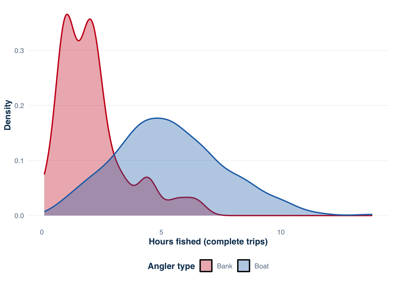
Figure 5.3: Distribution of completed trip durations (hours fished) at Harlan Reservoir, by angler type. Only complete trips are shown; incomplete trips are excluded from this display. Boat anglers fish longer trips on average than bank anglers, with a heavier right tail reflecting the greater logistical investment required to launch a boat.
Figure 5.3 shows the distribution of completed trip durations by angler type. Boat anglers tend to fish longer trips on average than bank anglers, with the boat distribution showing a heavier right tail — a pattern consistent with the greater investment required to launch and retrieve a boat, which creates an incentive to make the trip longer. This difference matters for effort estimation: if boat and bank anglers are counted together but have different mean trip durations, a single mean trip duration used in the estimator will be biased toward whichever type is more numerous in the interview sample on any given day.
The incomplete trips excluded from Figure 5.3 — those with trip_status == "incomplete" in the harlan_interviews table — represent anglers intercepted mid-trip and therefore cannot report total hours fished. Their proportion and distribution relative to complete trips is an important diagnostic for survey quality.
Species composition of harvest
What species did anglers harvest, and in what proportions?
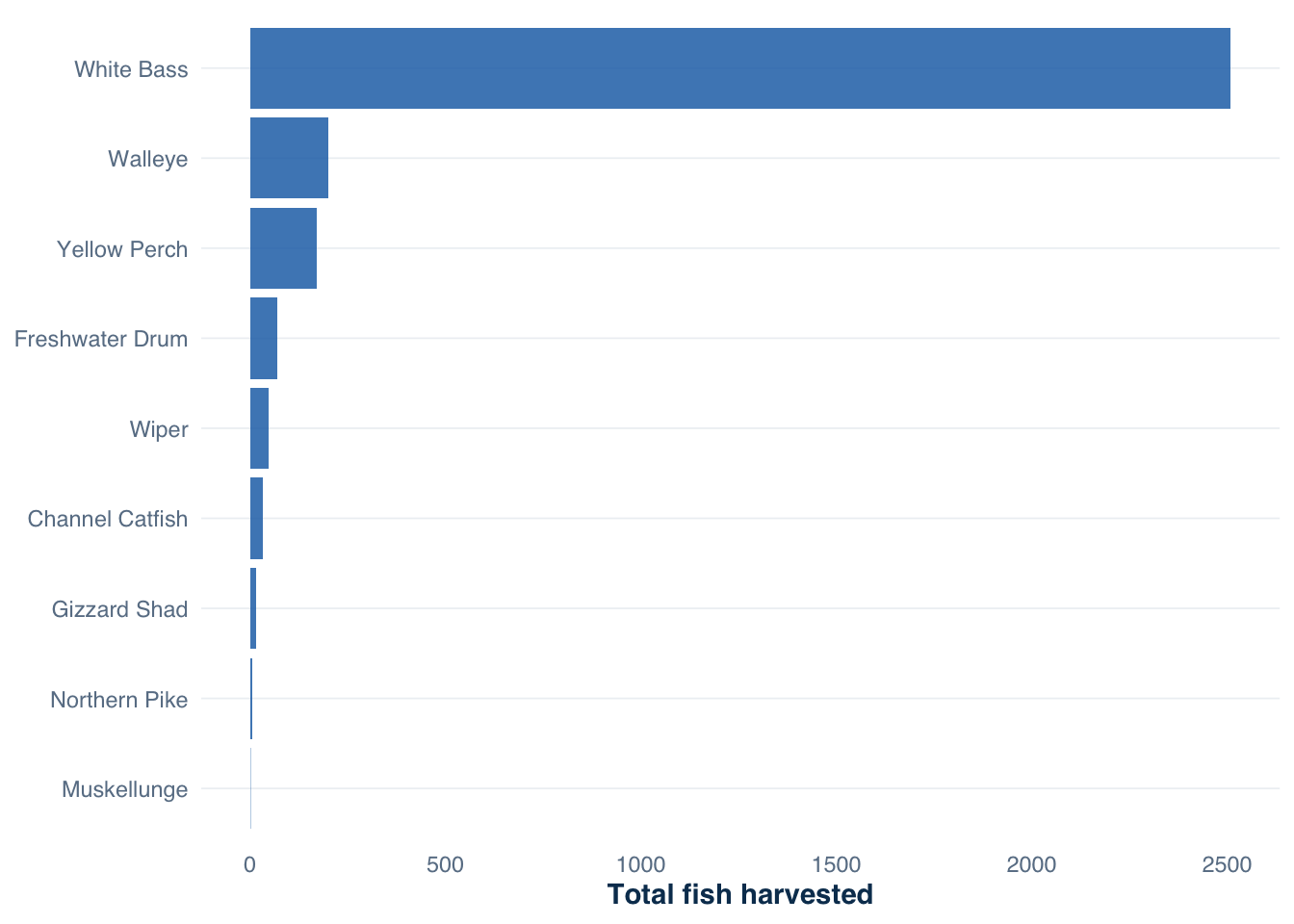
Figure 5.4: Total harvested fish by species at Harlan Reservoir across the 2022 survey season, ordered by total harvest. White Bass and Walleye account for the largest share of angler harvest; this is raw interview-reported harvest, not a design-weighted estimate.
Figure 5.4 shows the species composition of angler harvest across the season. This is raw interview-reported harvest, not a design-weighted estimate — it reflects what the interviewed anglers reported, not an expansion to the whole fishery. The full seasonal harvest estimate, which weights these records by the inverse probability of the day being sampled, is computed in Chapter 4. Comparing the raw interview totals to the design-weighted estimates is a useful diagnostic: large discrepancies suggest that the sampled days were not representative of the season as a whole, which may indicate design problems or unusually high-variance months.
The multi-species composition is typical of reservoir fisheries in the central plains. Warmwater reservoir surveys rarely target a single species; anglers mix their targeting opportunistically based on conditions, season, and access. An estimation pipeline that handles species-disaggregated harvest — separately for each species while sharing the common effort denominator — is therefore essential. tidycreel handles this through the estimate_total_harvest() function, which accepts a species grouping argument and produces estimates for each species in a single call.
5.10 Takeaway
Creel surveys are inferential tools, not counting exercises. The field records are a sample. The design is what authorizes the extrapolation. The estimand defines what the extrapolation is supposed to represent.
Three questions summarize what every creel analyst needs to answer before touching the data:
What is the claim? Which estimand, over which reporting domain, for which time period?
Does the design support the claim? Were the sampled days drawn from a frame that covers the reporting domain? Were the strata defined before sampling, not after?
Is the workflow reproducible? Can the estimate be traced back to source records, rerun when data change, and audited by someone who was not in the room when it was produced?
The rest of this book provides the methods to answer all three questions in R, using the Harlan Reservoir dataset as a consistent running example and formal theory as the foundation for every estimation function. But those methods are only as good as the design and the analytical discipline behind them. A well-implemented estimator applied to a poorly designed survey produces a precise estimate of the wrong thing.
Harmon, B. S., D. R. Martin, C. J. Chizinski, and K. L. Pope. 2018. Variation in angler distribution and catch rates of stocked rainbow trout in a small reservoir. PLOS ONE 13(1):e0190745.
Pollock, K. H., C. M. Jones, and T. L. Brown. 1994. Angler survey methods and their applications in fisheries management. American Fisheries Society, Bethesda, Maryland.
Pope, K. L., C. J. Chizinski, A. J. Lynch, and J. R. Post. in pressin press. Creel surveys.