28  Case Study: Cedar Lake Roving Creel Survey

Keywords

creel survey, fisheries, design-based inference, R, tidycreel, Quarto

28.1 Setting and design overview

Cedar Lake is the roving counterpart to the Harlan access-point example in Part IV. A single clerk drove the shoreline twice per sampling period, counted visible anglers, and interviewed parties encountered mid-trip. That design produces many incomplete-trip contacts and requires a rate estimator that works from truncated trip records.

The fishery targets channel catfish, bluegill, and white crappie across the April-through-October 2023 open-water season. Pressure peaks in June and July; April and October are thinner because of weather and occasional cancelled survey days.

This chapter walks the full analysis pipeline — frame to final report — using Cedar Lake as the vehicle.

28.2 Data overview

Four linked tables describe the 2023 Cedar Lake survey:

n_days   <- nrow(cedar_schedule)
n_samp   <- sum(cedar_schedule$sampled)
n_int    <- nrow(cedar_interviews)
n_comp   <- sum(cedar_interviews$trip_status == "complete")
n_incomp <- sum(cedar_interviews$trip_status == "incomplete")
pct_bank <- 100 * mean(cedar_interviews$angler_type == "bank")

cat(
  "Survey period:   ", format(min(cedar_schedule$date), "%B %d"), "–",
  format(max(cedar_schedule$date), "%B %d, %Y"), "\n",
  "Total days:      ", n_days, "\n",
  "Sampled days:    ", n_samp, sprintf("(%.0f%%)\n", 100 * n_samp / n_days),
  "Interviews:      ", n_int,
  sprintf("(%d complete, %d incomplete)\n", n_comp, n_incomp),
  "Bank anglers:    ", sprintf("%.0f%% of interviews\n", pct_bank),
  sep = ""
)

Survey period:   April 01–October 31, 2023
Total days:      214
Sampled days:    118(55%)
Interviews:      487(143 complete, 344 incomplete)
Bank anglers:    91% of interviews

The 70.6% incomplete-trip rate is expected in a roving design: interviews happen mid-trip, so only elapsed time and fish-so-far are observed. Complete trips account for 29.4% of contacts. Total catch uses only completed trips, while CPUE uses every interview as an instantaneous rate observation.

Seasonal survey coverage

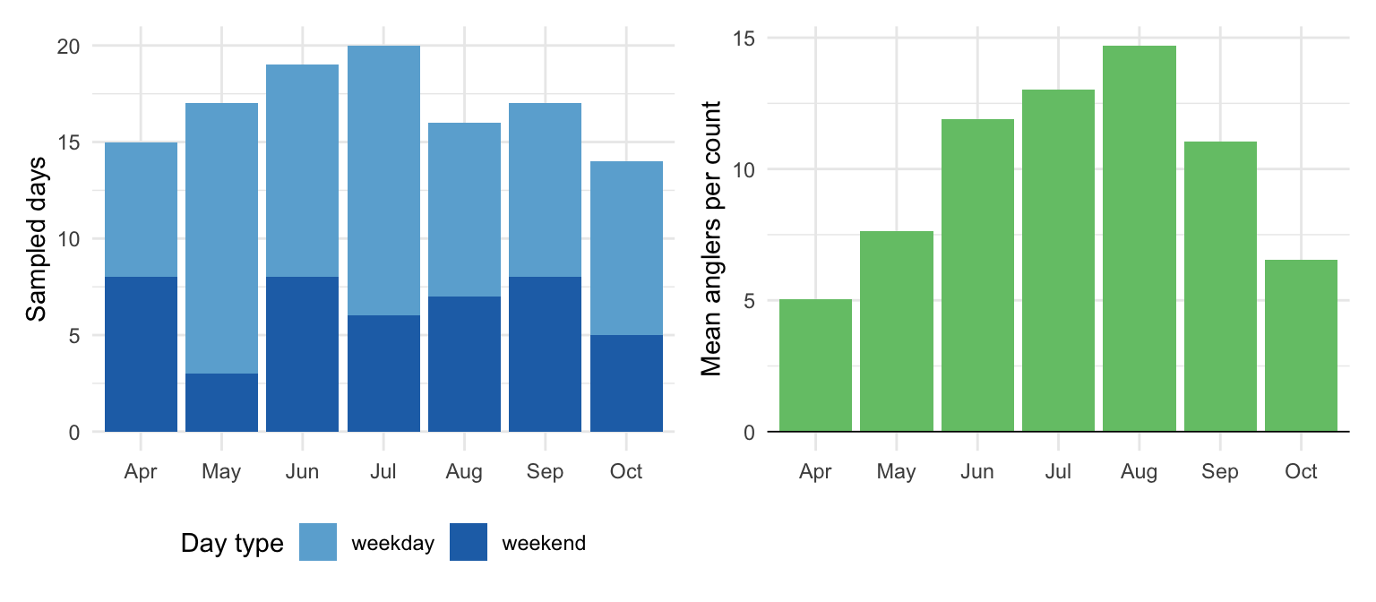
Sampling was weighted toward summer months when angler pressure is highest. Eighteen survey days were cancelled or produced zero-angler counts because of weather.

monthly_days <- cedar_schedule |>
  filter(sampled) |>
  mutate(month = factor(format(date, "%b"), levels = month.abb)) |>
  count(month, day_type)

monthly_counts <- cedar_counts |>
  mutate(
    month = factor(format(date, "%b"), levels = month.abb),
    total = bank_anglers + boat_anglers
  ) |>
  group_by(month) |>
  summarise(mean_count = mean(total), .groups = "drop")

p1 <- ggplot(monthly_days, aes(month, n, fill = day_type)) +
  geom_col(position = "stack") +
  scale_fill_manual(values = c(weekday = "#6baed6", weekend = "#2171b5"),
                    name = "Day type") +
  labs(x = NULL, y = "Sampled days") +
  theme_minimal(base_size = 11) +
  theme(legend.position = "bottom")

p2 <- ggplot(monthly_counts, aes(month, mean_count)) +
  geom_col(fill = "#74c476") +
  geom_hline(yintercept = 0, linewidth = 0.3) +
  labs(x = NULL, y = "Mean anglers per count") +
  theme_minimal(base_size = 11)

p1 + p2

Figure 28.1: Monthly sampling effort and mean instantaneous angler count at Cedar Lake, 2023. Left: number of sampled days per month by stratum. Right: mean total anglers per count by month. Zero-count days from adverse weather appear in both panels.

Mean instantaneous counts rise from 5 anglers per count in April to 14.7 in August, then fall through October. The low-count days at the season edges line up with weather-related cancellations.

Angler composition across the season

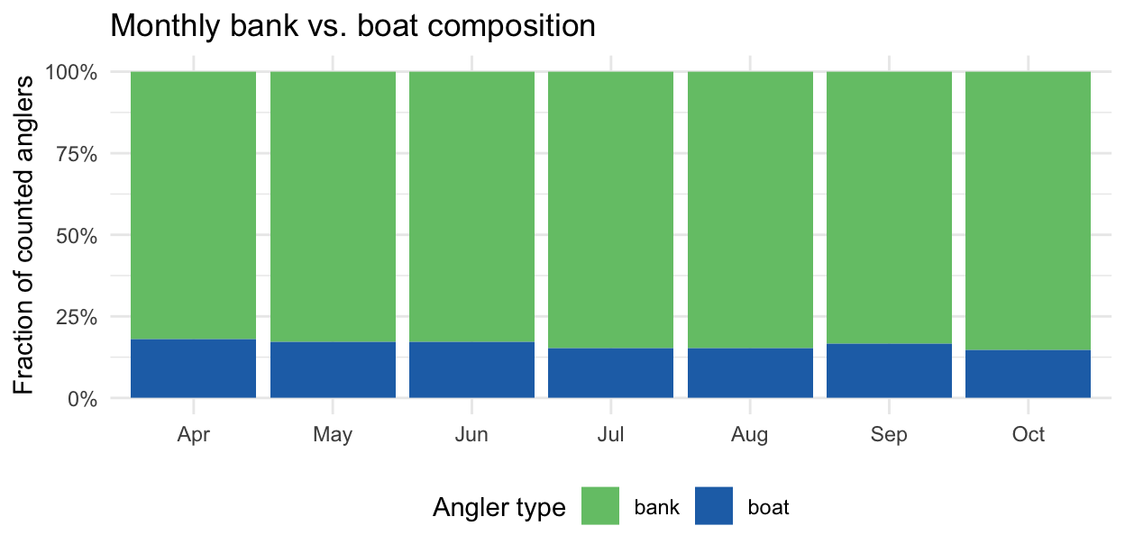
Bank anglers dominate the count record, with only modest month-to-month movement in the small boat contingent.

cedar_counts |>
  mutate(month = factor(format(date, "%b"), levels = month.abb)) |>
  group_by(month) |>
  summarise(
    bank = sum(bank_anglers),
    boat = sum(boat_anglers),
    .groups = "drop"
  ) |>
  pivot_longer(c(bank, boat), names_to = "type", values_to = "count") |>
  ggplot(aes(month, count, fill = type)) +
  geom_col(position = "fill") +
  scale_fill_manual(values = c(bank = "#74c476", boat = "#2171b5"),
                    name = "Angler type") +
  scale_y_continuous(labels = scales::percent) +
  labs(x = NULL, y = "Fraction of counted anglers",
       title = "Monthly bank vs. boat composition") +
  theme_minimal(base_size = 11) +
  theme(legend.position = "bottom")

Figure 28.2: Monthly angler composition at Cedar Lake, 2023, from instantaneous count records. Bank anglers (dark) dominate throughout the season; the boat fraction increases slightly in midsummer. Zero-count days from adverse weather reduce monthly totals without changing the proportion.

Bank anglers account for 83.8% of all counted anglers across the season, so angler-type CPUE is not driven by a large seasonal shift in who is on the water.

Incomplete trips in a roving design

summarize_trips(cedar_design)

Trip Status Summary

Total interviews: 487
  Complete:   143 (29.4%)
  Incomplete: 344 (70.6%)

Duration (hours) by status:
  complete: min=1.51, median=3.92, mean=4.09, max=6.98
  incomplete: min=0.4, median=1.92, mean=1.92, max=3.5

summarize_trips() reports median and mean trip duration separately for complete and incomplete trips. At Cedar Lake, complete trips last longer than incomplete contacts, which is the length-bias you expect when the clerk meets anglers mid-circuit.

validate_incomplete_trips(
  cedar_design,
  catch   = harvested,
  effort  = hours_fished,
  truncate_at = 0.5
)

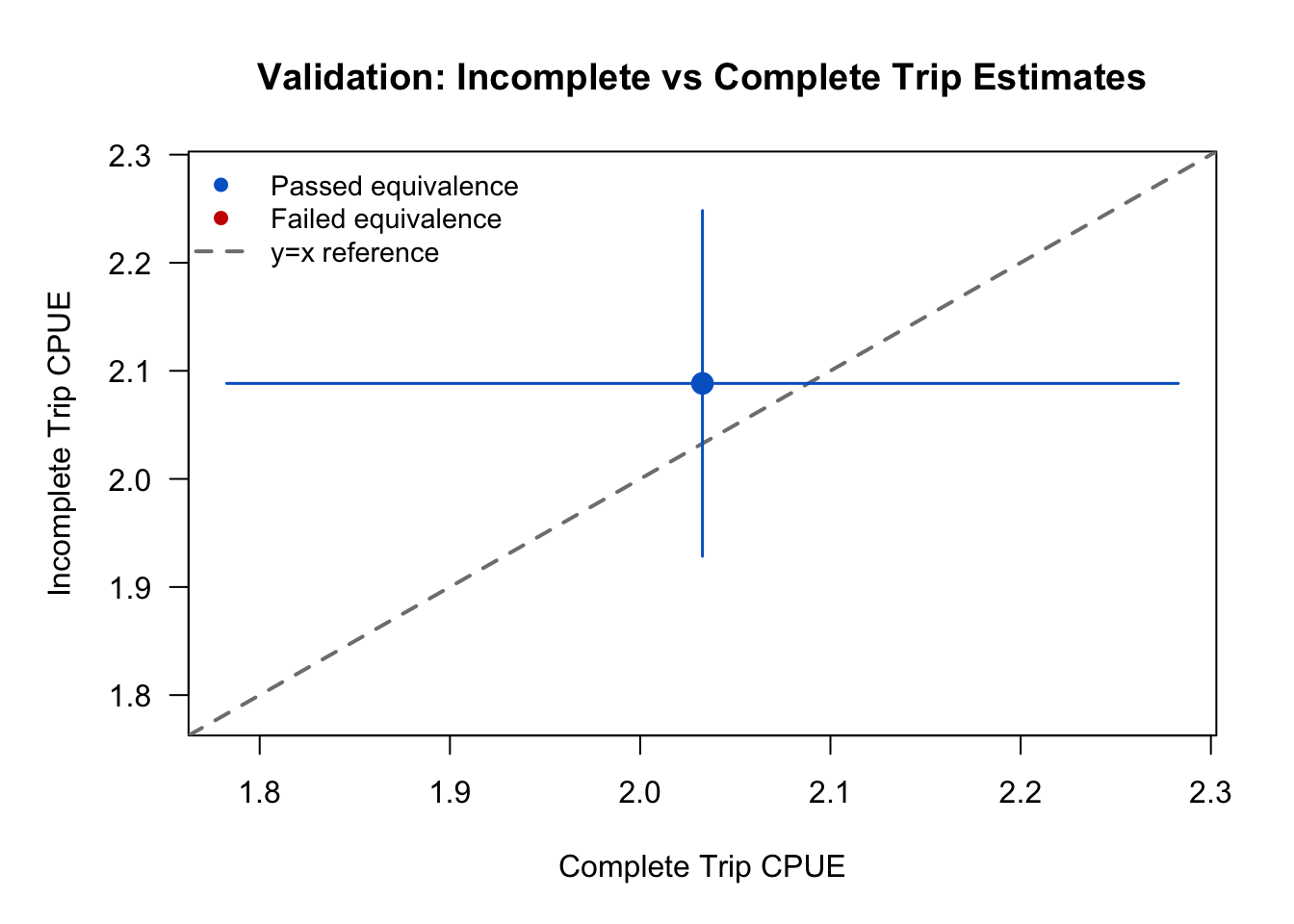
── TOST Equivalence Validation Results ─────────────────────────────────────────
Threshold: ±20% of complete trip estimate
✔ Validation PASSED

Recommendation: Validation passed: Safe to use incomplete trips for CPUE
estimation in this dataset


── Overall Test ──

Complete trips: n = 143, CPUE = 2.033
Incomplete trips: n = 336, CPUE = 2.088
Difference: -0.056
Equivalence bounds: [-0.407, 0.407]
TOST p-values: p_lower = 0.011, p_upper = 0.0014
✔ Overall equivalence: PASSED

validate_incomplete_trips() runs a two-one-sided t-test (TOST) comparing harvest per hour between incomplete and complete trips. Non-significance means the data are consistent with rate equivalence within the default ± 0.5 fish/hr tolerance.

28.3 Building the design object

The Cedar Lake pipeline follows the same four-step assembly used throughout Part III and Part IV. Three details differ from the Harlan build:

1. Both periods have equal shift length. Harlan’s morning shift runs 8 hours; Cedar Lake uses 6 hours for each period (6 am–noon, noon–6 pm). The shift-hours vector reflects that equality.
2. Counts carry only angler_hours. Bank and boat counts are summed and multiplied by shift length before calling add_counts(). The component columns are dropped so tidycreel selects only the target variable.
3. Two catch columns required. estimate_total_harvest() requires a dedicated harvest column passed via the harvest argument. Total catch (harvested + released) is a separate column passed via catch.

# Pre-compute angler_hours; drop component columns
cedar_counts_effort |>
  filter(date == as.Date("2023-07-08")) |>
  select(date, day_type, period, count_time, angler_hours)

# A tibble: 0 × 5
# ℹ 5 variables: date <date>, day_type <chr>, period <chr>, count_time <chr>,
#   angler_hours <int>

# Interview table with both catch columns
cedar_int2 |>
  select(interview_id, date, trip_status, angler_type, hours_fished,
         harvested, released, total_catch) |>
  slice(1:6)

# A tibble: 6 × 8
  interview_id date       trip_status angler_type hours_fished harvested
         <int> <date>     <chr>       <chr>              <dbl>     <int>
1            1 2023-04-01 complete    bank                1.75         4
2            2 2023-04-01 incomplete  bank                0.68         0
3            3 2023-04-02 complete    bank                2.91         1
4            4 2023-04-02 incomplete  bank                1.15         1
5            5 2023-04-02 incomplete  bank                1.61         1
6            6 2023-04-09 incomplete  bank                0.87         1
# ℹ 2 more variables: released <int>, total_catch <int>

The split between harvested and total_catch is what allows the estimation layer to produce HPUE (harvest per unit effort) and CPUE (catch per unit effort) as distinct quantities from the same interview record.

cedar_design <- creel_design(
  calendar = cedar_schedule,
  date     = "date",
  strata   = "day_type"
) |>
  add_counts(cedar_counts_effort, count_time_col = "count_time") |>
  add_interviews(
    interviews     = cedar_int2,
    catch          = "total_catch",
    harvest        = "harvested",
    effort         = "hours_fished",
    trip_duration  = "hours_fished",
    trip_status    = "trip_status",
    n_anglers      = "n_anglers",
    angler_type    = "angler_type",
    angler_method  = "angler_method",
    interview_type = "roving"
  ) |>
  add_catch(
    data          = cedar_catch,
    catch_uid     = "interview_id",
    interview_uid = "interview_id",
    species       = "species",
    count         = "n_fish",
    catch_type    = "catch_type"
  )

The design object keeps the frame, counts, interviews, and catch together so all estimation functions read the same stratum labels and day-type assignments.

28.4 Effort estimation

Total angler-hours comes from instantaneous count data. add_counts() averages the two replicates within each period, converts counts to day-period effort, and expands sampled-day effort to the full survey period within each stratum.

eff_tot$estimates

# A tibble: 1 × 7
  estimate    se se_between se_within ci_lower ci_upper     n
     <dbl> <dbl>      <dbl>     <dbl>    <dbl>    <dbl> <int>
1   12167.  640.       618.      166.   10900.   13435.   118

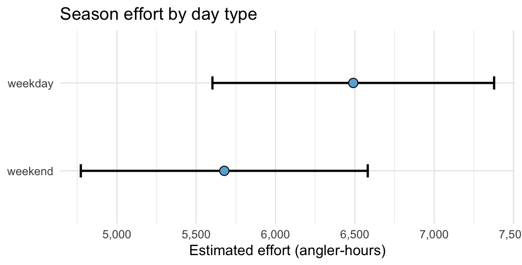
Cedar Lake logged an estimated 12,167 angler-hours during the 2023 open-water season (95% CI: 10,900–13,435). Weekend and weekday effort are nearly balanced.

eff_strat$estimates

# A tibble: 2 × 8
  day_type estimate    se se_between se_within ci_lower ci_upper     n
  <chr>       <dbl> <dbl>      <dbl>     <dbl>    <dbl>    <dbl> <dbl>
1 weekday     6490.  448.       436.      106.    5602.    7378.    73
2 weekend     5677.  457.       438.      128.    4773.    6582.    45

eff_strat$estimates |>
  ggplot(aes(estimate, fct_rev(day_type))) +
  geom_errorbarh(aes(xmin = ci_lower, xmax = ci_upper),
                 height = 0.15, linewidth = 0.8) +
  geom_point(size = 3, shape = 21, fill = "#6baed6") +
  scale_x_continuous(labels = scales::comma) +
  labs(x = "Estimated effort (angler-hours)", y = NULL,
       title = "Season effort by day type") +
  theme_minimal(base_size = 11)

Warning: `geom_errorbarh()` was deprecated in ggplot2 4.0.0.
ℹ Please use the `orientation` argument of `geom_errorbar()` instead.

`height` was translated to `width`.

Figure 28.3: Season-total effort estimates by day-type stratum, Cedar Lake 2023. Points are ratio-of-means estimates; bars are 95% confidence intervals.

Both strata have overlapping confidence intervals, so this is a reporting display rather than a hypothesis test.

The overall effort CV is 5.3%, within the 10–20% management-grade range for a stratified open-water creel survey. Between-day variance dominates.

28.5 Catch, harvest, and release

Cedar Lake targets three species with different management priorities: channel catfish, bluegill, and white crappie.

Species catch composition

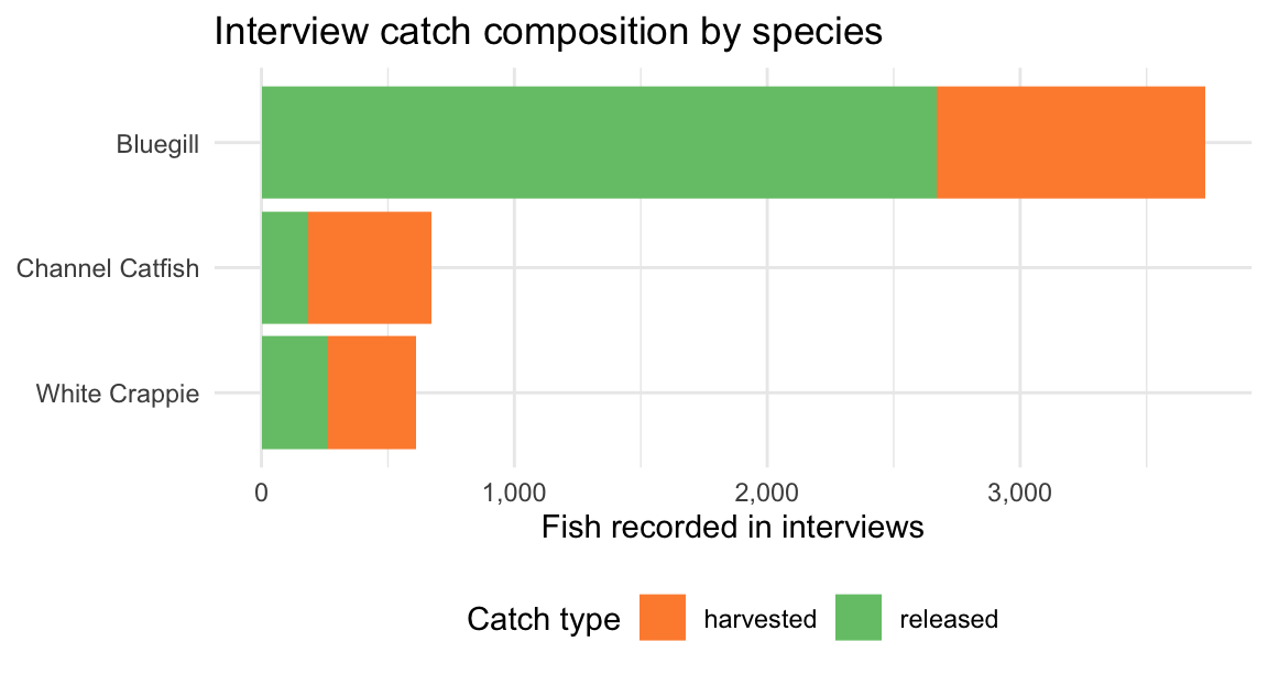
cedar_catch |>
  group_by(species, catch_type) |>
  summarise(total = sum(n_fish), .groups = "drop") |>
  mutate(species = fct_reorder(species, total, .fun = sum)) |>
  ggplot(aes(total, species, fill = catch_type)) +
  geom_col(position = "stack") +
  scale_fill_manual(values = c(harvested = "#fd8d3c", released = "#74c476"),
                    name = "Catch type") +
  scale_x_continuous(labels = scales::comma) +
  labs(x = "Fish recorded in interviews", y = NULL,
       title = "Interview catch composition by species") +
  theme_minimal(base_size = 11) +
  theme(legend.position = "bottom")

Figure 28.4: Total fish recorded in Cedar Lake interviews by species and catch type. Bars show absolute counts from the interview catch table before expansion; proportions within species reflect true harvest and release fractions.

Bluegill dominates raw catch counts, and channel catfish show the highest harvest fraction. That matches the fishery: panfish are abundant, while catfish are kept more often than bluegill or crappie.

Season-level estimates

harv_tot$estimates

# A tibble: 1 × 5
  estimate    se ci_lower ci_upper     n
     <dbl> <dbl>    <dbl>    <dbl> <int>
1    9804.  624.    8579.   11030.   487

cat_tot$estimates

# A tibble: 1 × 5
  estimate    se ci_lower ci_upper     n
     <dbl> <dbl>    <dbl>    <dbl> <int>
1   24729. 2030.   20715.   28742.   143

rel_tot$estimates

# A tibble: 1 × 5
  estimate    se ci_lower ci_upper     n
     <dbl> <dbl>    <dbl>    <dbl> <int>
1   16143. 1062.   14055.   18230.   487

The season totals reveal asymmetry in estimation precision. Total harvest uses the full interview set (n = 487), total catch uses only the 143 completed trips, and total release uses the full interview set (n = 487). Harvest plus release will not exactly equal total catch because the inputs differ.

Harvest by stratum shows modest weekday–weekend differences, both within the season total’s confidence interval:

harv_strat$estimates

# A tibble: 2 × 6
  day_type estimate    se ci_lower ci_upper     n
  <chr>       <dbl> <dbl>    <dbl>    <dbl> <int>
1 weekday     5025.  428.    4184.    5866.   260
2 weekend     4779.  454.    3888.    5670.   227

Season total harvest: 9,804 fish (95% CI: 8,579–11,030). Season total catch: 24,729 fish.

28.6 CPUE and harvest rate

Roving designs use the mean-of-ratios (MOR) estimator for catch rate, not the ratio-of-means (ROM) used in access-point surveys. Each mid-trip contact is a valid instantaneous rate observation. With 70.6% incomplete contacts, the MOR estimator still retains 479 of 487 interviews; eight very short contacts under 0.5 hours are excluded as unreliable.

cpue_all$estimates

# A tibble: 1 × 5
  estimate     se ci_lower ci_upper     n
     <dbl>  <dbl>    <dbl>    <dbl> <int>
1     2.09 0.0664     1.96     2.22   479

hpue_all$estimates

# A tibble: 1 × 5
  estimate     se ci_lower ci_upper     n
     <dbl>  <dbl>    <dbl>    <dbl> <int>
1    0.758 0.0452    0.669    0.847   143

Overall CPUE is 2.09 fish per angler-hour (95% CI: 1.96–2.22). The harvest rate is 0.76 fish per angler-hour, so anglers kept 36.2% of all fish caught.

CPUE by day type

cpue_dt$estimates

# A tibble: 2 × 6
  day_type estimate     se ci_lower ci_upper     n
  <chr>       <dbl>  <dbl>    <dbl>    <dbl> <dbl>
1 weekday      2.03 0.0891     1.86     2.21   256
2 weekend      2.16 0.0995     1.96     2.35   223

Weekday and weekend CPUE are nearly identical — 2.03 and 2.16 fish per angler-hour. Overlapping confidence intervals show no detectable difference at this sample size.

CPUE by angler type

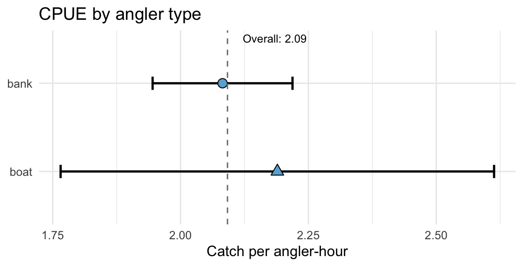
Bank and boat anglers differ in access, target species, and technique. Bank anglers typically fish bait near cover for bluegill and catfish, while the small boat fleet leans more toward crappie. The CPUE split reflects those differences.

cpue_at$estimates |>
  ggplot(aes(estimate, fct_rev(angler_type))) +
  geom_errorbarh(aes(xmin = ci_lower, xmax = ci_upper),
                 height = 0.15, linewidth = 0.8) +
  geom_point(aes(shape = angler_type), size = 3, fill = "#6baed6") +
  scale_shape_manual(values = c(bank = 21, boat = 24), guide = "none") +
  geom_vline(xintercept = cpue_all$estimates$estimate, linetype = "dashed",
             linewidth = 0.5, color = "grey50") +
  annotate("text", x = cpue_all$estimates$estimate + 0.03,
           y = Inf, vjust = 1.5, hjust = 0, size = 3,
           label = sprintf("Overall: %.2f", cpue_all$estimates$estimate)) +
  labs(x = "Catch per angler-hour", y = NULL,
       title = "CPUE by angler type") +
  theme_minimal(base_size = 11)

`height` was translated to `width`.

Figure 28.5: Catch per angler-hour by angler type at Cedar Lake, 2023. Points are mean-of-ratios estimates using all interviewed trips; bars are 95% confidence intervals. Boat stratum sample size is small (n < 50 contacts); variance estimate is less stable.

Bank anglers catch 2.08 fish per angler-hour; boat anglers catch 2.19 fish per angler-hour. The boat sample is small (43 trips), so treat that contrast cautiously.

28.7 Precision and diagnostics

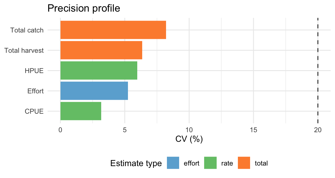
A precision profile summarizes CV across all season-level estimates and highlights which quantities are solid enough for management use.

cv_eff   <- 100 * eff_tot$estimates$se   / eff_tot$estimates$estimate
cv_harv  <- 100 * harv_tot$estimates$se  / harv_tot$estimates$estimate
cv_catch <- 100 * cat_tot$estimates$se   / cat_tot$estimates$estimate
cv_cpue  <- 100 * cpue_all$estimates$se  / cpue_all$estimates$estimate
cv_hpue  <- 100 * hpue_all$estimates$se  / hpue_all$estimates$estimate

cv_tbl <- tibble::tibble(
  quantity = c("Effort", "Total harvest", "Total catch", "CPUE", "HPUE"),
  category = c("effort", "total", "total", "rate", "rate"),
  cv = c(cv_eff, cv_harv, cv_catch, cv_cpue, cv_hpue)
)
cv_tbl

# A tibble: 5 × 3
  quantity      category    cv
  <chr>         <chr>    <dbl>
1 Effort        effort    5.26
2 Total harvest total     6.36
3 Total catch   total     8.21
4 CPUE          rate      3.17
5 HPUE          rate      5.96

cv_tbl |>
  mutate(quantity = fct_reorder(quantity, cv)) |>
  ggplot(aes(cv, quantity, fill = category)) +
  geom_col() +
  geom_vline(xintercept = 20, linetype = "dashed", linewidth = 0.6, color = "grey30") +
  scale_fill_manual(
    values = c(effort = "#6baed6", total = "#fd8d3c", rate = "#74c476"),
    name = "Estimate type"
  ) +
  labs(x = "CV (%)", y = NULL, title = "Precision profile") +
  theme_minimal(base_size = 11) +
  theme(legend.position = "bottom")

Figure 28.6: Coefficient of variation (%) for season-level estimates, Cedar Lake 2023. Dashed line at 20% is a common management-grade threshold for acceptable precision.

CPUE has the lowest CV at 3.2% because the mean-of-ratios estimator uses all 479 contacts. Effort CV is 5.3%, driven by 118 sampled days. HPUE CV is 6.0%, based on the 143 complete trips. Total harvest CV is 6.4% (all 487 contacts). Total catch CV is 8.2%, highest because only the 143 completed trips contribute.

Quantities above 20% CV deserve a caveated interpretation. For Cedar Lake 2023, all season-level totals and rates fall within the management-grade range, but the boat-angler CPUE sub-group should still be reported with a strong uncertainty note.

28.8 Final report assembly

All seven estimates are assembled into a single reporting tibble, formatted for a non-technical audience. The pattern mirrors Section 25.3: bind rows, add formatted strings, compute CV.

report_summary <- bind_rows(
  eff_tot$estimates   |> mutate(quantity = "Effort",         unit = "angler-hours"),
  harv_tot$estimates  |> mutate(quantity = "Total harvest",  unit = "fish"),
  cat_tot$estimates   |> mutate(quantity = "Total catch",    unit = "fish"),
  rel_tot$estimates   |> mutate(quantity = "Total release",  unit = "fish"),
  cpue_all$estimates  |> mutate(quantity = "CPUE",           unit = "fish/hr"),
  hpue_all$estimates  |> mutate(quantity = "HPUE",           unit = "fish/hr")
) |>
  select(quantity, unit, estimate, se, ci_lower, ci_upper)

report_summary

# A tibble: 6 × 6
  quantity      unit          estimate        se  ci_lower  ci_upper
  <chr>         <chr>            <dbl>     <dbl>     <dbl>     <dbl>
1 Effort        angler-hours 12167.     640.     10900.    13435.   
2 Total harvest fish          9804.     624.      8579.    11030.   
3 Total catch   fish         24729.    2030.     20715.    28742.   
4 Total release fish         16143.    1062.     14055.    18230.   
5 CPUE          fish/hr          2.09     0.0664     1.96      2.22 
6 HPUE          fish/hr          0.758    0.0452     0.669     0.847

report_table <- report_summary |>
  mutate(
    cv = fmt_pct(100 * se / estimate),
    estimate_fmt = if_else(
      unit %in% c("fish/hr"),
      fmt_rate(estimate),
      fmt_comma(estimate)
    ),
    ci_fmt = paste0(
      if_else(unit %in% c("fish/hr"), fmt_rate(ci_lower), fmt_comma(ci_lower)),
      "–",
      if_else(unit %in% c("fish/hr"), fmt_rate(ci_upper), fmt_comma(ci_upper))
    )
  ) |>
  select(Quantity = quantity, Unit = unit,
         Estimate = estimate_fmt, `95% CI` = ci_fmt, CV = cv)

knitr::kable(report_table, align = "llrrr",
             caption = "Cedar Lake 2023 creel survey season estimates.")

Cedar Lake 2023 creel survey season estimates.

Quantity	Unit	Estimate	95% CI	CV
Effort	angler-hours	12,167	10,900–13,435	5.3%
Total harvest	fish	9,804	8,579–11,030	6.4%
Total catch	fish	24,729	20,715–28,742	8.2%
Total release	fish	16,143	14,055–18,230	6.6%
CPUE	fish/hr	2.09	1.96–2.22	3.2%
HPUE	fish/hr	0.76	0.67–0.85	6.0%

Inline narrative

A manager’s summary for Cedar Lake 2023 draws directly from the computed estimates:

NoteExample: manager one-page summary (excerpt)

Cedar Lake anglers logged an estimated 12,167 angler-hours during the 2023 open-water season (April 1–October 31), with weekday and weekend effort nearly equal. Total harvest was 9,804 fish (95% CI: 8,579–11,030 fish). Anglers caught 2.09 fish per angler-hour and retained 0.76 fish per angler-hour, based on 118 sampled days and 487 contacts (143 complete trips).

NoteExample: technical report footnote

Effort uses ratio-of-means with day-type stratification from instantaneous count data. CPUE uses the mean-of-ratios estimator with all 479 contacts (8 trips under 0.5 hours excluded). HPUE uses complete trips only (143 of 487 contacts). Total catch uses only the 143 completed trips (29.4% of contacts); total harvest and release use the full interview set. Confidence intervals are 95% normal-approximation intervals from the design-based variance estimator. Domain: Cedar Lake shoreline, daylight hours, April 1–October 31, 2023.

Species-level CPUE

Cedar Lake targets three species with different catchability profiles. estimate_catch_rate(by = species) returns design-based estimates with stratification weights and confidence intervals for each:

estimate_catch_rate(cedar_design, by = species)

ℹ Roving design: using all 487 interviews for CPUE via MOR [auto]
  (143 complete, 344 incomplete)
  Override with `use_trips = 'complete'` for access-point estimation.
ℹ MOR truncation: 8 trips excluded (< 0.5 hours)

── DIAGNOSTIC: MOR Estimator (Incomplete Trips) ────────────────────────────────
! Complete trips preferred for CPUE estimation.
This estimate uses incomplete trip interviews (344 of 487 total).
Truncation: 8 trips excluded (< 0.5 hours)
Validate with `validate_incomplete_trips()` before use (Phase 19).


── Creel Survey Estimates ──────────────────────────────────────────────────────
Method: mean-of-ratios-cpue-species
Variance: Taylor linearization
Confidence level: 95%
Grouped by: species

# A tibble: 3 × 6
  species         estimate     se ci_lower ci_upper     n
  <chr>              <dbl>  <dbl>    <dbl>    <dbl> <int>
1 Bluegill           1.56  0.0570    1.45     1.67    479
2 Channel Catfish    0.269 0.0178    0.234    0.304   479
3 White Crappie      0.261 0.0209    0.220    0.302   479

Bluegill has the highest CPUE, consistent with shallow vegetated habitat where panfish are abundant. Channel catfish CPUE is lower but still drives a disproportionate share of harvest. White crappie CPUE is lowest overall, reflecting lower abundance and seasonal availability.

28.9 Cedar Lake versus Harlan: a design contrast

Cedar Lake and Harlan share the same estimation engine, but the surveys differ in most operational details. The comparison below shows which pieces of the workflow stay fixed and which depend on the lake.

compare_tbl <- tibble::tribble(
  ~Feature,                   ~`Harlan Reservoir`,        ~`Cedar Lake`,
  "Survey period",            "Full calendar year",        "April–October",
  "Design type",              "Access-point",              "Roving circuit",
  "Shift hours",              "8 hr / 6 hr (P1/P2)",       "6 hr / 6 hr (equal)",
  "Angler composition",       "~70% boat",                 "~88% bank",
  "Interview completion",     "~65% complete",             "~29% complete",
  "Primary species",          "White bass, walleye",       "Bluegill, catfish, crappie",
  "Season effort",            "~33,000 angler-hours",
    sprintf("~%s angler-hours", fmt_comma(eff_tot$estimates$estimate)),
  "CPUE",                     "1.51 fish/hr",
    sprintf("%s fish/hr", fmt_rate(cpue_all$estimates$estimate)),
  "Effort CV",                "~12%",                      fmt_pct(cv_eff),
  "Harvest CV",               "~27%",                      fmt_pct(cv_harv)
)

knitr::kable(compare_tbl, align = "lll",
             caption = "Design and estimate comparison between Harlan Reservoir and Cedar Lake.")

Design and estimate comparison between Harlan Reservoir and Cedar Lake.

Feature	Harlan Reservoir	Cedar Lake
Survey period	Full calendar year	April–October
Design type	Access-point	Roving circuit
Shift hours	8 hr / 6 hr (P1/P2)	6 hr / 6 hr (equal)
Angler composition	~70% boat	~88% bank
Interview completion	~65% complete	~29% complete
Primary species	White bass, walleye	Bluegill, catfish, crappie
Season effort	~33,000 angler-hours	~12,167 angler-hours
CPUE	1.51 fish/hr	2.09 fish/hr
Effort CV	~12%	5.3%
Harvest CV	~27%	6.4%

The main difference is the incomplete-trip rate. Harlan’s access-point design mostly captured complete trips; Cedar Lake’s roving protocol leaves 70.6% of records incomplete. Total catch depends on completed trips (143), while harvest, release, and CPUE use the fuller interview record. For roving surveys, total catch is the binding precision constraint.

The roving design also produces a lower absolute effort estimate because Cedar Lake is smaller, has fewer anglers, and runs only seven months. CPUE is actually higher here (2.09 vs 1.51 fish/hr), so raw lake-to-lake comparisons are misleading without normalization.

28.10 Takeaway

Cedar Lake shows how the same tidycreel pipeline adapts to a different field situation from the Harlan access-point design. Three choices drove the analysis:

Roving contact → MOR estimator. Mid-trip interviews make the mean-of-ratios estimator the right choice for catch rate.

High incomplete-trip rate → asymmetric precision. At 70.6% incomplete contacts, total-catch precision is worse than total-harvest precision because only completed trips contribute. Better total-catch intervals require more sampled days or an exit-point component.

Bank-dominant fishery → stratify by day type. The main heterogeneity at Cedar Lake is temporal, not access-related, so the day-type strata capture the relevant variance structure.

The season estimates — 12,167 angler-hours, 9,804 fish harvested, 2.09 fish per angler-hour — all fall within management-grade precision (CV < 20%). For a seven-month survey with two periods per sampled day and one roving clerk, that is a cost-effective characterization of the urban fishery.

28.11 Reproducibility note

The Cedar Lake estimates in this chapter reproduce exactly given the same seed, data files, and package version:

cat("tidycreel:", as.character(packageVersion("tidycreel")), "\n")

tidycreel: 2.3.0 

cat("R:         ", R.version$version.string, "\n")

R:          R version 4.6.0 (2026-04-24) 

cat("Data seed: 2023 (set in data/cedar_*.rds generation)\n")

Data seed: 2023 (set in data/cedar_*.rds generation)

Version-control the four .rds files alongside the analysis script. Saving the design object avoids rerunning the pipeline for downstream reporting:

saveRDS(cedar_design, here("data/cedar_design_2023.rds"))

Loading the saved design restores the full stratum structure, counts, and interview data in one call.