creel survey, fisheries, design-based inference, R, tidycreel, Quarto
21.1 Why effort comes first
Every estimate produced by a creel survey is either effort itself or a product that uses effort as a scaling factor. If effort is wrong, every downstream number built on it is wrong too.
Effort estimation therefore sits at the foundation of the creel workflow. The count schedule — which days to sample, how many periods per day, how many instantaneous counts per period — is determined by the precision requirements for effort, not by the requirements for catch rate or harvest. Getting effort right means understanding what the instantaneous count estimator targets, how stratification turns counts into a season total, and where variance comes from.
This chapter works through effort estimation for the Harlan Reservoir 2022 survey: the formula that converts an instantaneous angler count into an angler-hour total, the stratified expansion that converts sampled days into a full-season estimate, the variance decomposition that separates between-day uncertainty from within-day uncertainty, and the estimate_effort() function in tidycreel that assembles all of these pieces in a single call.
21.2 What effort means in a creel survey
Creel surveys measure effort as the amount of fishing activity in a defined domain over a defined time period. That simple statement still requires three explicit choices before any arithmetic can begin.
The unit of effort. Angler-hours — one angler fishing for one hour — is the most common unit in North American inland fisheries (Pollock et al. 1994). It is natural for the instantaneous count estimator because an angler count at a point in time, multiplied by the length of the fishing period, gives angler-hours directly. Some designs count boats rather than individual anglers and report boat-hours, then convert to angler-hours using a mean party size from the interview record. Harlan records both boat_anglers (individual anglers on boats) and bank_anglers (shore anglers), so the natural unit is total angler-hours from all modes combined.
The domain. The domain specifies what population the estimate covers — which water, which species, which access modes, which time of day. The Harlan schedule covers a single reservoir section (section = "0") surveyed over two daily shifts (morning period 1 and afternoon period 2) from April through October 2022. Effort estimated from Harlan counts represents fishing pressure within that section-shift-season domain; extrapolation beyond it requires assumptions that the data cannot support.
The reporting period. Managers typically want a seasonal or annual total, not just effort on sampled days. The stratified estimator expands from sampled days to the full calendar. That expansion rests on an assumption: sampled days within a stratum are representative of all days in that stratum. The sampling design is responsible for making this assumption defensible; stratification by day type (weekday vs. weekend) reduces the risk by keeping groups with different effort levels in separate strata.
Fishing pressure on a given day-period can also be reported as angler-trips rather than angler-hours. An angler-trip counts each party as one unit regardless of how long they fish; it answers “how many trips happened” rather than “how much fishing time was expended.” Angler-hours and angler-trips measure different things and can diverge substantially when trip lengths vary — a fishery dominated by long overnight trips has fewer trips but more hours than one dominated by quick half-day outings. Which unit a manager needs depends on the question being asked.
21.3 The instantaneous count estimator
An instantaneous count records the number of anglers active in the survey area at a single moment in time. Multiplying by the length of the fishing period converts a count to an angler-hour estimate for that period (Pope et al. in press):
\hat{E}_{d,p} = \bar{I}_{d,p} \times T_p
where \hat{E}_{d,p} is the estimated angler-hours on day d during period p, \bar{I}_{d,p} is the mean of the K_{d,p} instantaneous counts taken within that period, and T_p is the total length of the period in hours. The mean rather than the sum of counts is used because each count estimates the instantaneous stock of anglers, not a cumulative total; averaging multiple counts within a period reduces the effect of moment-to-moment fluctuation.
At Harlan, morning shifts (period 1) run 8 hours and afternoon shifts (period 2) run 6 hours, with two instantaneous counts per shift. For the morning of September 2, 2022, the two counts recorded 38 and 45 boat anglers (no bank anglers active):
The 332 angler-hours estimated for that single morning shift illustrates the scale of the effort signal. A sampled period with 41.5 mean anglers and an 8-hour shift contributes more than three person-days of fishing activity to the seasonal total.
Why two counts, not one?
With only one count per period, the daily effort estimate has no within-period variance and the analyst cannot assess how much moment-to-moment fluctuation exists in angler activity (McCormick et al. 2013). Two counts allow estimation of within-day variance, which is a component of total effort variance. The recommendation from McCormick et al. (2013) is to take at least two counts per period, spread across the shift, so that the within-day variance can be estimated and included in the uncertainty budget.
At Harlan, the two counts per period are separated by approximately two hours, providing coverage of both the early-shift and mid-shift activity levels. The add_counts() call in tidycreel records both counts, averages them to a single period-day mean, and retains the within-day variance for inclusion in estimate_effort() output.
21.4 Stratified expansion to the season total
Effort on sampled days must be expanded to the full survey period to produce the seasonal total managers need. The stratified expansion works by scaling the stratum sample mean up to the stratum population size (Rasmussen et al. 1998):
where N_h is the number of days available in stratum h (from the sampling calendar), n_h is the number of days actually sampled, and the sum runs over sampled days s_h. The ratio N_h / n_h is the expansion weight: it says “each sampled day in this stratum represents N_h / n_h days in the population.”
The overall season estimate sums across strata:
\hat{E} = \sum_h \hat{E}_h
For Harlan, the sampling calendar covers 211 days (April 2 to October 29, 2022), divided into weekday (N_{\text{weekday}} = 150) and weekend (N_{\text{weekend}} = 61) strata. Of these, 82 weekday days and 34 weekend days were sampled. Each sampled day is assigned to one shift — either morning (period 1, 8 hours) or afternoon (period 2, 6 hours) — giving 118 period-day records in the count data (83 weekday + 35 weekend).
Weekdays are sampled at a slightly lower rate than weekends (55% vs. 56%), but the stratum sizes are very different: 150 weekday days vs. 61 weekend days. The weekend stratum is smaller in both total days and sampled days, which matters for precision — smaller strata with fewer sampled days produce wider confidence intervals even when their sampling fraction is similar.
The daily estimator versus the stratum estimator
Two estimators for seasonal effort appear in the creel literature, and they behave differently in practice. Rasmussen et al. (1998) compared them directly using simulation on the Escanaba Lake dataset.
The daily estimator(Malvestuto et al. 1978) first computes a mean daily effort for the full sampling period and then multiplies by the total number of days:
\hat{E}_{\text{daily}} = N \cdot \frac{1}{n} \sum_{d=1}^{n} \hat{E}_d
This estimator ignores stratum membership and treats all sampled days as interchangeable. When effort differs systematically between weekdays and weekends — as it almost always does — the daily estimator will be biased if sampled days are not proportionally distributed across day types. Random variation in day-type representation across the sample can produce large positive or negative swings in the estimate.
The stratum estimator(Rasmussen et al. 1998) estimates effort separately within each stratum and then sums. It is unbiased regardless of how day-type composition varies across the sample, because weekday and weekend days contribute to their respective stratum means independently. Rasmussen et al. demonstrated that the stratum estimator produced bias ratios near zero across 1,000 simulations, while the daily estimator showed substantially larger deviations from census values in years with low overall effort. All effort estimates in this chapter use the stratum estimator.
21.5 Variance of the effort estimate
The variance of a stratified effort estimate has two distinct sources, and understanding their magnitudes guides decisions about survey design (McCormick et al. 2013).
Between-day variance is the variance in daily effort across sampled days within a stratum. It reflects genuine day-to-day variation in how many anglers fish — driven by weather, season, weekday patterns, and stochastic factors. The between-day variance estimator for stratum h is the standard stratified sampling result with a finite population correction:
where s_{E,h}^2 is the sample variance of daily effort estimates across sampled days in stratum h. This term dominates when days differ widely in angler activity — common for weekend strata where a rainy October weekend and a sunny June weekend can have an order-of-magnitude difference in effort.
Within-day variance is the variance across multiple instantaneous counts taken within a single period. It reflects moment-to-moment fluctuation in angler presence during the shift: anglers departing for lunch, boats moving between sites, brief periods of low activity following a weather event. The within-day variance contribution is:
where K_d is the number of counts on day d and s_d^2 is their sample variance. With only two counts per period-day, this is just T_p^2 \cdot
(c_1 - c_2)^2 / 2.
estimate_effort() reports both components as se_between and se_within, making it straightforward to determine which source of uncertainty is more important. When se_between dominates, increasing the number of sampled days reduces uncertainty more than adding count rounds within already sampled days. When se_within dominates — rare in practice but possible in highly variable systems — adding within-day count rounds is the more efficient path (McCormick et al. 2013).
21.6 Preparing count data for effort estimation
The estimate_effort() function operates on whatever numeric column comes first in the design’s count data that is not a date, strata, or sampling unit identifier. For Harlan, the raw count table records bank_anglers, angler_boats, and boat_anglers separately. Passing these columns directly would cause estimate_effort() to estimate effort in units of bank anglers alone — the first numeric column — rather than in total angler-hours.
The correct workflow is to hand add_counts() the untransformed count together with the shift length, and let it do the conversion:
Code
# Shift lengths for each periodshift_hours <-c("1"=8L, "2"=6L)harlan_counts_effort <- harlan_counts |>mutate(period =as.character(period), # prevent period from being treated as a count# add_counts() scales the count and the party-size basis together via# period_length_col. Multiplying the count here instead would leave# expansion_basis in the old units and understate the party-size term.shift_length = shift_hours[period] ) |>select( reservoir, date, day_type, period, section, count_time, angler_count, shift_length, expansion_basis, expansion_se, expansion_group, expansion_of )harlan_counts_effort |>filter(date ==as.Date("2022-09-02")) |>select(date, day_type, period, count_time, angler_count, shift_length)
Two things happen here. First, period is converted from numeric to character so that estimate_effort() does not interpret it as a count variable (period values of 1 and 2 are identifiers, not observations). Second, the shift length is attached as a column rather than multiplied into the count, and period_length_col tells add_counts() to apply it. The multiplication has to happen inside add_counts() because expansion_basis is the derivative of the count with respect to party size: scaling the count outside the function leaves the basis in the old units and silently understates the party-size variance component. add_counts() then averages the two within-period records to a single period-day mean — matching the formula \bar{I}_{d,p} \times T_p at the data preparation stage rather than in the estimator.
The full design pipeline with effort-preprocessed counts:
Warning in svydesign.default(ids = psu_formula, strata = strata_formula, : No
weights or probabilities supplied, assuming equal probability
Warning: 318 interviews have zero catch.
ℹ Zero catch may be valid (skunked) or indicate missing data.
Warning: ! Catch totals in catch data diverge from interview-level total_harvest for 329
  interviews.
ℹ This is advisory. Real creel data may differ legitimately (partial species
  recording).
The design holds the same survey structure built in Section 19.1 — calendar, strata, interviews, catch — but the counts slot now carries angler_count scaled to angler-hours as its single numeric count variable, with the design’s effort_unit recording that unit. This ensures all downstream effort estimates are in angler-hours rather than raw angler counts.
21.7 Effort on sampled days
estimate_effort() returns effort for the sampled days only when target = "sampled_days" (the default). This is the design-weighted sum of angler-hours actually observed across all sampled period-day combinations, without extrapolating to unsampled days.
Warning: Count variable angler_count contains 18 zero values.
ℹ Zero values may indicate days with no fishing activity or data collection
  issues.
ℹ Consider whether zeros are true zeros or missing data.
Warning: Count variable expansion_basis contains 21 zero values.
ℹ Zero values may indicate days with no fishing activity or data collection
  issues.
ℹ Consider whether zeros are true zeros or missing data.
Code
eff_sampled
── Creel Survey Estimates ──────────────────────────────────────────────────────
Method: Total
Variance: Taylor linearization
Confidence level: 95%
Effort target: sampled_days
Unit: angler-hours
Party-size expansion SE: 489.9 (included in se)

# A tibble: 1 × 7
  estimate    se se_between se_within ci_lower ci_upper     n
     <dbl> <dbl>      <dbl>     <dbl>    <dbl>    <dbl> <int>
1   21678. 2538.      2247.     1073.   16651.   26705.   118
The 118 sampled period-days produced 2.168e+04 observed angler-hours, with a standard error of 2,538 angler-hours (CV = 11.7%). This is not a seasonal estimate — it covers only the periods that were actually surveyed — but it benchmarks the observed effort against which the full-season expansion can be compared.
The SE decomposes into a between-day component of 2,247 angler-hours and a within-day component of 1,073 angler-hours. Between-day variance accounts for the larger share: day-to-day differences in how many anglers visit Harlan are a more important source of uncertainty than moment-to-moment fluctuation within a shift. This is the typical pattern for reservoir fisheries where weather and seasonality drive large swings in daily attendance.
21.8 Full-season effort estimate
The primary management deliverable is the full-season angler-hour estimate — expanded from sampled days to the complete sampling frame using the stratum weights N_h / n_h. The target = "stratum_total" argument applies this expansion:
Warning: Count variable angler_count contains 18 zero values.
ℹ Zero values may indicate days with no fishing activity or data collection
  issues.
ℹ Consider whether zeros are true zeros or missing data.
Warning: Count variable expansion_basis contains 21 zero values.
ℹ Zero values may indicate days with no fishing activity or data collection
  issues.
ℹ Consider whether zeros are true zeros or missing data.
Code
eff_season
── Creel Survey Estimates ──────────────────────────────────────────────────────
Method: Total
Variance: Taylor linearization
Confidence level: 95%
Effort target: stratum_total
Unit: angler-hours
Party-size expansion SE: 880.7 (included in se)

# A tibble: 1 × 7
  estimate    se se_between se_within ci_lower ci_upper     n
     <dbl> <dbl>      <dbl>     <dbl>    <dbl>    <dbl> <int>
1   38969. 3182.      2697.     1441.   32667.   45270.   118
Expanding to all 211 calendar days yields an estimated 3.897e+04 angler-hours for the Harlan 2022 season (April–October), with a 95% confidence interval of approximately 3.267e+04 to 4.527e+04 angler-hours. The CV of 8.2% satisfies the commonly cited 20% target for management-grade estimates (McCormick et al. 2013), though it falls in the range that some agencies consider acceptable rather than comfortable.
The ratio of stratum_total to sampled_days reflects the proportion of the season that was surveyed. Harlan sampled 55% of available days (116 of 211), so the expansion factor is approximately 1.82. The actual expansion differs slightly between strata because weekday and weekend days were sampled at slightly different rates.
21.9 Effort by stratum
The four-cell breakdown by day type and period reveals how effort is distributed across the sampling frame:
Warning: Count variable angler_count contains 18 zero values.
ℹ Zero values may indicate days with no fishing activity or data collection
  issues.
ℹ Consider whether zeros are true zeros or missing data.
Warning: Count variable expansion_basis contains 21 zero values.
ℹ Zero values may indicate days with no fishing activity or data collection
  issues.
ℹ Consider whether zeros are true zeros or missing data.
Three patterns are immediately visible. First, weekday effort substantially exceeds weekend effort in every period — weekday morning effort alone (1.866e+04 angler-hours) is larger than total weekend effort across both periods. This is the reverse of the pattern typical for urban-access reservoirs and reflects Harlan’s location in rural south-central Nebraska, where mid-week fishing by retirees, nearby residents, and agricultural workers is common.
Second, morning effort (period 1) exceeds afternoon effort (period 2) for both day types. Morning periods are 8 hours long versus 6 hours for afternoons, but the count-per-unit-time is also higher in the morning, so the difference reflects genuine differences in angler behavior rather than just shift-length arithmetic.
Third, the weekend strata carry wider confidence intervals relative to their estimates (higher CV). The weekend stratum has fewer sampled days and more variable day-to-day attendance — sunny summer weekends draw large crowds while cold autumn weekends can be nearly empty — so the between-day variance is larger relative to the mean.
The marginal day-type totals collapse across periods:
Warning: Count variable angler_count contains 18 zero values.
ℹ Zero values may indicate days with no fishing activity or data collection
  issues.
ℹ Consider whether zeros are true zeros or missing data.
Warning: Count variable expansion_basis contains 21 zero values.
ℹ Zero values may indicate days with no fishing activity or data collection
  issues.
ℹ Consider whether zeros are true zeros or missing data.
Code
eff_daytype
── Creel Survey Estimates ──────────────────────────────────────────────────────
Method: Total
Variance: Taylor linearization
Confidence level: 95%
Grouped by: day_type
Effort target: stratum_total
Unit: angler-hours
Party-size expansion SE: 753.8 and 126.9 (included in se)

# A tibble: 2 × 8
  day_type estimate    se se_between se_within ci_lower ci_upper     n
  <chr>       <dbl> <dbl>      <dbl>     <dbl>    <dbl>    <dbl> <int>
1 weekday    33346. 3001.      2553.     1385.   27403.   39289.    83
2 weekend     5623.  963.       868.      397.    3715.    7530.    35
Weekdays account for 86% of total estimated angler-hours (3.335e+04 AH) against 14% for weekends (5,623 AH). This split has direct management implications: a regulation targeting weekend fishing pressure would affect a minority of total season effort, while a midweek closure would affect the majority.
21.10 Seasonal pattern in effort
The survey calendar spans April through October. Within that window, effort is not evenly distributed — spring and early summer typically see higher fishing pressure than late fall. The mean angler-hours per sampled period-day by month describes this seasonal arc directly from the observed counts:
Warning: No shared levels found between `names(values)` of the manual scale and the
data's fill values.
No shared levels found between `names(values)` of the manual scale and the
data's fill values.
No shared levels found between `names(values)` of the manual scale and the
data's fill values.
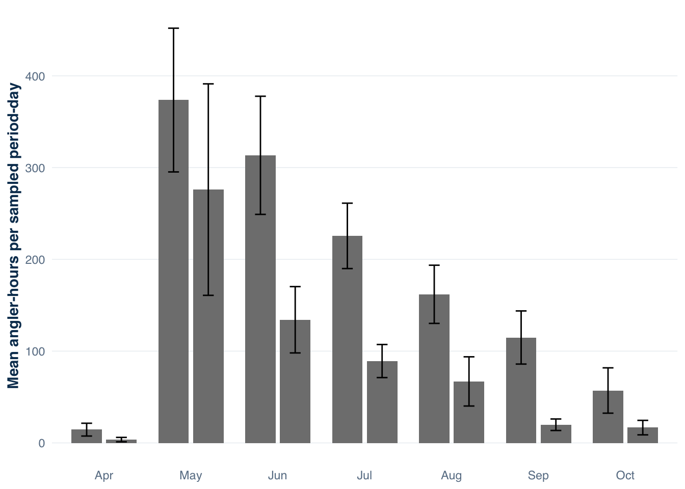
Figure 21.1: Mean angler-hours per sampled period-day by month and day type, Harlan Reservoir 2022. Each bar represents the average of all sampled period-days within a month-day-type combination; error bars show one standard error. The survey covers April through October. Weekday effort (dark) consistently exceeds weekend effort (light) across the season; both peak in May and decline through autumn.
May records the highest mean effort on sampled period-days for both day types, with weekday mornings averaging over 300 angler-hours. This likely reflects the opening of the main spring fishing season at Harlan — walleye and white bass are highly targeted in May — combined with the long spring days that extend the productive morning period. Effort declines through summer and into autumn, with October weekday averages roughly one-fifth of the May peak.
The April values are near zero because most April sampled days fell in early April before anglers had established regular patterns. This emphasizes a practical point: sampled days near the margins of the season carry a disproportionate share of the between-day variance (a zero-effort day and a 300-angler-hour day in the same stratum drive a large s_{E,h}^2). If the calendar boundary is set too early or too late relative to when fishing actually occurs, the expansion weights amplify this edge-effect noise into the seasonal total.
21.11 Stratum-level effort estimates with confidence intervals
The point estimates and uncertainty intervals for the full-season breakdown visualize which strata carry the most effort and where estimation uncertainty is largest:
Warning: No shared levels found between `names(values)` of the manual scale and the
data's fill values.
No shared levels found between `names(values)` of the manual scale and the
data's fill values.
No shared levels found between `names(values)` of the manual scale and the
data's fill values.
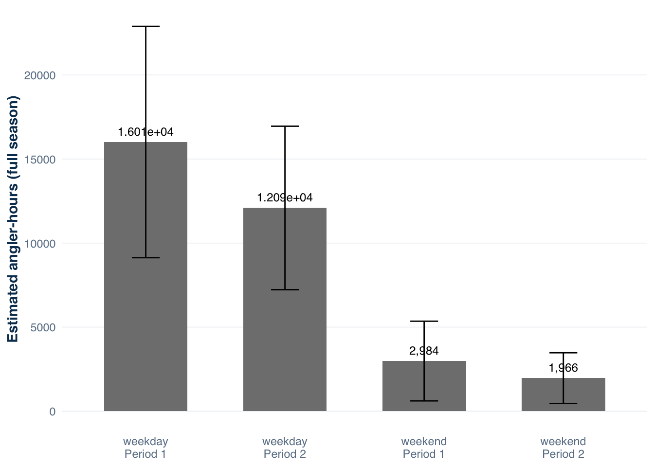
Figure 21.2: Estimated full-season angler-hours by day type and period, Harlan Reservoir 2022. Bars show the stratum_total estimate (expanded to all calendar days in each stratum). Error bars show 95% confidence intervals from the Taylor linearization variance estimator. Numbers above bars show the point estimate in angler-hours. Weekday mornings (period 1) dominate; weekend effort in either period is a small fraction of weekday effort.
The confidence intervals reveal why survey design decisions matter. The weekday period 1 CI spans roughly 14,000 angler-hours — a range large enough to affect management conclusions if the estimate were used to compare against a target fishing pressure threshold. The weekend period 2 CI is narrower in absolute terms but represents a similar proportional uncertainty because weekend effort is inherently lower. Reducing these intervals requires increasing the number of sampled days, not adding more count rounds per already-sampled day — because between-day variance dominates across all strata.
21.12 Precision and reporting
The coefficient of variation for the full-season estimate is 8.2%. Whether this is adequate depends on how the estimate will be used. For detecting year-over-year trends of 20–30%, a CV of 10–15% is generally sufficient because the trend signal is larger than the noise. For detecting changes of 10% or less — common when managing regulated fisheries close to exploitation targets — a CV below 10% is preferable (McCormick et al. 2013).
The standard error decomposes into between-day and within-day components:
Between-day variance accounts for 72% of total variance. Adding a third count round to already-sampled days would reduce the within-day component but leave the dominant between-day component unchanged. The most efficient way to reduce overall uncertainty is to sample more days — either by extending the survey season or by increasing the sampling fraction within existing strata.
Survey programs that want explicit precision targets before the season can use the variance decomposition from historical data to plan sample sizes. If prior surveys show s_{E,h}^2 for each stratum and the target CV is 15%, the required n_h follows directly from the standard stratified sampling formula (McCormick et al. 2013).
21.13tidycreel support
Implemented for instantaneous count designs:
estimate_effort() — stratified effort estimator with Taylor variance, between/within decomposition, multiple targets (sampled_days, stratum_total, period_total), and grouping via by
estimate_effort_grouped() — called internally by estimate_effort() when by is specified
add_counts() with count_time_col — averages multiple within-period counts to a single period-day mean and computes within-day variance contribution
Constraints and workflow notes:
The count variable used by estimate_effort() is always the first numeric column in the design’s count data that is not a date, strata, or PSU column. Pass the count in its original units and name the shift-length column with period_length_col; add_counts() scales the count and the party-size basis together. Multiplying the count beforehand is refused, because the basis would be left in the old units.
Convert period (and any similar integer identifiers) to character before calling add_counts() to prevent them from being selected as count variables.
The stratum_total target requires that the design have a strata column and that the calendar cover the full survey period. Days not in the calendar cannot be expanded to.
Not in scope for this chapter:
Bus-route effort estimation — handled by estimate_effort_br(), covered in Section 9.1 but not demonstrated here
Aerial and camera-trap designs — handled by estimate_effort_aerial() and estimate_effort_camera(), introduced in Section 11.1
Sample size planning — requires external calculation using variance estimates from this chapter as inputs; tidycreel does not currently provide an optimal_n() function (see TIDYCREEL-WISHLIST.md)
21.14 Takeaway
Effort estimation is the point of the count schedule and the foundation for every harvest and catch total the survey produces. Getting it right means three things.
First, the instantaneous count estimator assumes that each count represents the instantaneous angler stock during the period. That assumption holds when counts are taken at random or representative times within the period. Counts clustered at the same time of day — always at 9:00 a.m., always at midday — can produce biased effort estimates if angler activity peaks and valleys are systematic.
Second, stratification by day type is not optional decoration. Without it, the random day-to-day composition of the sample can produce large swings in the estimated total. With it, weekday and weekend effort are estimated from samples of their respective populations, and the expansion to the full season is unbiased regardless of how any particular week was sampled.
Third, between-day variance almost always dominates. The lesson for survey design is that sampling more days per season is more effective than adding count rounds to days already sampled. A second or third count round per shift reduces within-day noise, but if days vary substantially in effort — as they do at any reservoir influenced by weather and season — only more days can reduce the dominant between-day component.
The Harlan 2022 season estimate of approximately 3.897e+04 angler-hours (95% CI 3.267e+04–4.527e+04) is the number that Section 22.1 will use to scale harvest and catch totals. The downstream confidence intervals are wider because effort uncertainty multiplies through \hat{E} \times \hat{R}.
Malvestuto, S. P., W. D. Davies, and W. L. Shelton. 1978. An evaluation of the roving creel survey with nonuniform probability sampling. Transactions of the American Fisheries Society 107(2):255–262.
McCormick, J. L., M. C. Quist, and D. J. Schill. 2013. Creel survey design considerations for short-duration fisheries with applications to Chinook salmon sport fisheries. North American Journal of Fisheries Management 33(3):628–641.
Pollock, K. H., C. M. Jones, and T. L. Brown. 1994. Angler survey methods and their applications in fisheries management. American Fisheries Society, Bethesda, Maryland.
Pope, K. L., C. J. Chizinski, A. J. Lynch, and J. R. Post. in pressin press. Creel surveys.
Rasmussen, P. W., M. D. Staggs, T. D. Beard, and S. P. Newman. 1998. Bias and confidence interval coverage of creel survey estimators evaluated by simulation. Transactions of the American Fisheries Society 127:469–480.