creel survey, fisheries, design-based inference, R, tidycreel, Quarto
10.1 Why roving surveys exist
The access-point design in Chapter 4 rests on a tractable assumption: anglers pass through a finite, enumerable set of entry and exit points. That assumption holds well for a reservoir with one boat ramp and a small bank-fishing area. It fails for a 100-kilometer river reach where anglers can reach the water from road bridges, wading accesses, and unimproved shore landings at hundreds of points. No finite roster of clerks can staff every entry. The access-point frame is incomplete by construction.
Roving surveys were developed for exactly this setting (Pollock et al. 1994). Rather than waiting for anglers to come to a fixed station, a clerk moves through the fishery — by boat, by vehicle, or on foot — and records what they encounter. Counts of anglers on the water supply the effort estimate. Interviews conducted while anglers are still fishing supply the catch rate estimate. Total catch is the product of the two, not a direct observation.
The design has become the most widely used on-site creel method in North American fisheries management (Pollock et al. 1994, Ch. 15), despite posing statistical challenges that the access-point design avoids. The central challenge is that roving interviews happen mid-trip. The angler has not finished fishing, the clerk does not know how long the trip will last, and the fraction of the trip already observed is an incomplete record of what the completed trip will contain. Handling that incompleteness correctly requires a different set of estimators than those used for completed trips.
This chapter works through roving survey design from first principles: how effort is estimated from counts, how mid-trip interviews produce catch rates through the mean-of-ratios estimator, where the design is vulnerable to bias, and how tidycreel supports the roving workflow. The running example is the Harlan Reservoir 2022 dataset. Harlan was operated primarily as an access-point survey, but the dataset includes 210 incomplete-trip interviews collected during mid-day roving contacts — enough to illustrate every feature of the roving analysis.
The short version is that roving surveys trade convenience for reach. They can cover anglers who never pass a fixed access point, but the analyst has to reconstruct the trip from partial information instead of from a finished record.
10.2 How roving surveys differ from access-point surveys
The structural difference between roving and access-point surveys is not where the clerk is stationed — it is when the interview happens relative to the trip.
In an access-point survey, the clerk waits at a fixed location and interviews anglers as they exit the fishery. Every interview is a completed trip. The angler reports total catch and total effort for the finished trip, and those reports feed directly into the ratio-of-means estimator developed in Chapter 4. Effort is also estimated from counts at the access point, so both components of the estimate come from the same fixed location.
In a roving survey, the clerk finds anglers during their trip. The interview captures catch so far and elapsed time so far — both of which are partial. Counts of anglers on the water record how many parties are active at the moment of the count, but those counts say nothing about how much time each angler will eventually log. Effort cannot be inferred from the interview record; it must be estimated separately from the count data. That separation — counts for effort, interviews for catch rate — is the defining feature of the roving design.
A roving survey operates two sampling processes simultaneously:
Counts are scheduled independently of interviews. A clerk following a circuit records every angler they can see at a defined time or across a defined route. These counts feed the effort estimator.
Interviews are collected in the gaps between counts, or in designs that separate counting and interviewing roles, by a second team. These interviews feed the catch rate estimator.
In practice the two processes are often collapsed onto a single clerk, creating operational pressure on both. The clerk who stops to conduct a thorough interview cannot simultaneously maintain a count of all anglers in sight. Understanding that the two processes serve different statistical purposes helps clarify when that trade-off matters and when it does not.
10.3 The sampling frame for a roving survey
The sampling frame for a roving survey is defined by routes, not by fixed stations. A route is a traversal path through the survey area — a lake circuit, a river reach, a sequence of shore segments — that can be replicated across survey days. What makes a route a frame element is that it covers a defined portion of the fishery with a known traversal time, so that an angler encountered during the route has a calculable probability of having been observed.
Frame design for roving surveys involves two decisions that have no direct analogue in access-point design:
Spatial coverage. The route must cover the fishery completely enough that every angler has a nonzero probability of being counted. In practice, complete spatial coverage is difficult on large water bodies, and routes are designed to capture representative transects rather than full censuses. Bias enters when parts of the fishery systematically avoid the route — a distant cove, an upstream tributary, a nighttime site not included in the daylight circuit.
Temporal scheduling. Count times must be scheduled across the full fishing day. An instantaneous count scheduled only at 9 a.m. captures the morning peak but misses afternoon use. Temporal stratification — scheduling some counts early and some late — distributes the count times across the day and prevents the effort estimate from depending entirely on whatever activity happened to coincide with a single observation window.
The Harlan survey frame covers a single primary access section (section = "0") over 211 days divided into morning (period 1) and afternoon (period 2) strata. Two instantaneous counts are conducted per sampled period, spaced approximately two hours apart. This design is not a roving circuit; it is a modified access-point design with multiple within-period count repetitions. The important point is that the same data structure — multiple count times per period at known observation points — supports the same effort estimation logic used in roving designs.
10.4 Counting anglers: instantaneous and progressive counts
Effort estimation in a roving survey begins from counts of anglers at specific moments or along specific traversal paths. Two count methods are in common use, and they produce different estimates because they sample different regions of the time-space plane that describes angling activity.
Instantaneous counts
An instantaneous count records the number of anglers active in the survey area at a single point in time. The clerk stops, counts every angler visible in the survey area, and records the total. That count, multiplied by the length of the fishing period, gives the estimated effort for the period:
\hat{E}_{\text{inst}} = n_t \times T
where n_t is the instantaneous count at time t and T is the total length of the fishing period in hours. If the count is taken at a random time during the period, this estimator is unbiased for period effort under the assumption that the number of anglers in the survey area is constant across the period — an assumption that is rarely exactly true but that averages out when count times are randomized.
When multiple instantaneous counts are available within a period, the effort estimate uses the average count:
\hat{E}_{\text{inst}} = \bar{n} \times T = \frac{1}{K} \sum_{k=1}^{K} n_k \times T
where K is the number of counts and \bar{n} is the mean count across count times. Averaging over multiple counts within a period reduces the effect of moment-to-moment fluctuation in angler activity.
Pierce and Bindman (1994) showed that instantaneous counts matched full-census effort estimates closely in a small lake study, validating the method for contained water bodies. For larger fisheries where complete instantaneous enumeration is impractical, the instantaneous count is taken at a defined point or transect rather than over the full water body, and the resulting effort estimate reflects only the fraction of the fishery covered.
The following code computes effort from the two instantaneous counts taken during the morning period on September 2, 2022, at Harlan Reservoir:
The two counts recorded 38 and 45 boat anglers (no bank anglers active on this morning), giving a mean of 41.5 anglers. Multiplied by the 8-hour morning shift, this yields:
Mean count: 46.32764 anglers
 Period length: 8 hours
 Estimated effort: 370.6211 angler-hours
The 332 angler-hours estimated for this one morning shift illustrates the scale of effort at Harlan. Extrapolated across all 116 sampled days, the seasonal effort total reaches into the tens of thousands of angler-hours — all derived from counts of instantaneous angler presence, never from direct summation of individual trip lengths.
The per-period effort estimates across the Harlan season reveal the difference between morning and afternoon use patterns:
Morning periods (period 1) averaged higher effort than afternoon periods (period 2) on both weekdays and weekends. Weekday mornings carry the highest average effort at Harlan — a pattern that likely reflects the reservoir’s distance from major urban centers and its use by retirees and local anglers who fish mid-week.
Progressive counts
A progressive count records anglers encountered while moving through the survey area rather than at a single moment. The clerk travels a defined route — a circuit of the lake by boat, a stretch of river by vehicle — and counts every angler they pass. An angler is included in the count if they are active when the clerk passes their location.
The distinction from an instantaneous count is geometric. An instantaneous count takes a vertical cross-section through time: all anglers active at moment t. A progressive count takes a diagonal cross-section through time and space: all anglers whose trips overlap the clerk’s path through the fishery. Hoenig et al. (1993) illustrate this with a figure showing nine hypothetical angler trips as horizontal lines in time-space. An instantaneous count at time t catches all trips extending through that moment. A progressive count starting at location 0 and ending at location S catches trips that overlap the diagonal path of the clerk.
Whether the instantaneous or progressive count produces a more precise effort estimate depends on the geometry of the fishery and the correlation between angler activity and location within the survey area. On a long river reach where anglers are spread across distinct segments, a progressive count that traverses the reach may be more representative than a single instantaneous count taken at one point. On a compact lake where the full surface is visible from one vantage point, an instantaneous count is simpler to execute and easier to replicate.
The effort estimator for a progressive count follows the same general form as the instantaneous estimator: count encountered \times period length. The key complication is that the count accumulates over a route traversal that takes real time, so the analyst must account for the fact that some anglers encountered early in the route may have finished by the time the route ends. Methods for handling this are described in Pollock et al. (1994, Ch. 11) and are closely related to the bus-route effort estimator developed in Chapter 4.
10.5 The incomplete-trip problem
Every roving interview records an angler in the middle of a trip. The angler started fishing at some time before the interview and will continue fishing for some time afterward. What the interview captures is the portion of the trip that had already elapsed at the moment of contact.
This creates a censoring problem. The analyst observes catch-so-far and effort-so-far, but not the trip’s eventual catch and duration. The ratio of catch-so-far to effort-so-far — the mid-trip catch rate — is not the same as the ratio of completed-trip catch to completed-trip effort. It equals the completed-trip rate only if fish are caught at a constant rate throughout the trip (stationary catch rate). That constancy assumption is rarely defensible: anglers move, feeding activity changes with light and temperature, and successful anglers either quit early when they reach a bag limit or fish longer to maximize harvest.
The key point is that the interview captures a moving target. A party that has already fished for two hours may still fish for four more, and a party that has fished for two hours may stop almost immediately. The observed ratio is real, but it is only a partial record of the trip.
The Harlan dataset reflects the incomplete-trip problem directly. Of 600 total interviews, 210 are flagged as incomplete — 35% of the interview record:
Code
harlan_interviews |>count(trip_status) |>mutate(pct =round(100* n /sum(n), 1))
# A tibble: 2 × 3
  trip_status     n   pct
  <chr>       <int> <dbl>
1 complete      390    65
2 incomplete    210    35
Incomplete trips are a feature, not an anomaly. They represent real contacts with real anglers that contain useful information. The analyst’s job is to use that information correctly — which requires choosing an estimator matched to the incomplete-trip structure.
10.6 Length-of-stay bias
Length-of-stay bias is intrinsic to the roving design. A clerk moving through a fishery is more likely to encounter an angler who has been fishing for a long time than one who has just started or is about to leave. The probability that a randomly timed contact finds angler j in the water is proportional to the length of angler j’s completed trip, L_j^*(Pollock et al. 1994, Ch. 11).
This oversampling of long trips has two consequences for inference.
Consequence 1: Overrepresentation of long-trip anglers. If catch rate, species targeted, and angling method all vary systematically with trip length, the interview sample will be dominated by anglers whose characteristics are not representative of the full population of trips. Successful anglers who linger to maximize catch are oversampled; anglers who leave early after a frustrating session are undersampled.
Consequence 2: Upward bias in observed trip duration. The elapsed time at interview is not the same as the completed trip duration. On average, a randomly timed contact intercepts an angler at the midpoint of their trip. Mean elapsed time at interview — which is what the analyst observes — will be approximately half the mean completed trip length if trips are distributed uniformly through the fishing day. The mean observed duration for incomplete trips at Harlan confirms this:
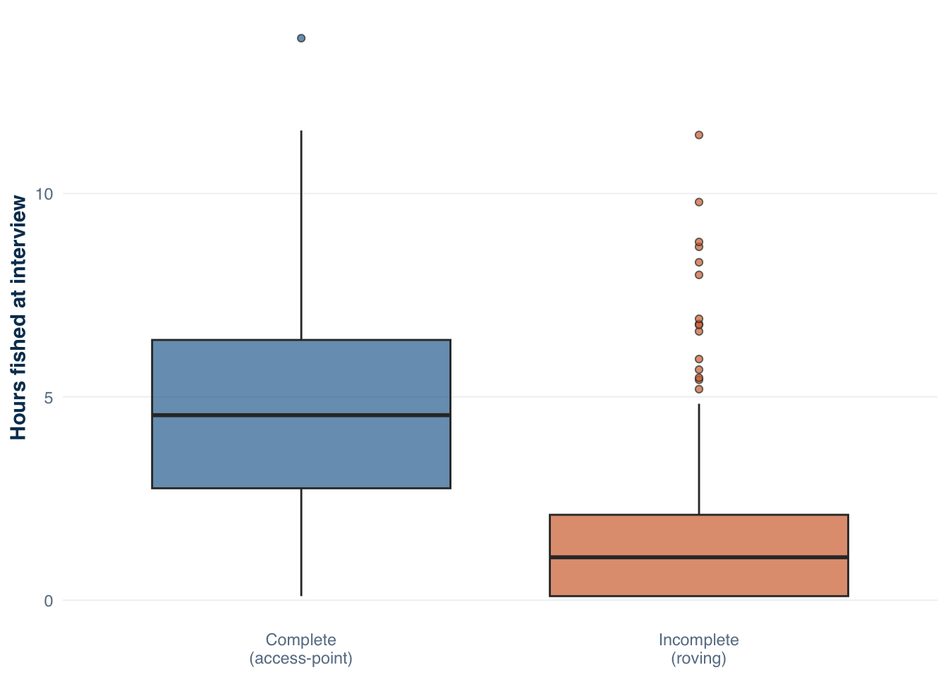
Completed trips at Harlan averaged 4.74 hours. Incomplete trips averaged 1.71 hours, about 36% of the completed-trip mean rather than 50%, reflecting that the distribution of trip start times is not uniform and that some anglers were contacted early in the morning shift before they had been out long.
Figure 10.1: Distribution of hours fished by trip status at Harlan Reservoir, 2022. Completed trips (access-point interviews) average 4.74 hours. Incomplete trips (roving contacts) average 1.71 hours — not because roving anglers fish less, but because roving contacts intercept trips mid-course. The gap illustrates why elapsed-time from incomplete interviews cannot substitute for completed-trip duration in effort estimation.
Avidity bias is a related but distinct problem. Anglers who fish more frequently — those who make many trips per season — are more likely to be encountered on any given survey day than infrequent anglers, regardless of trip length. This oversamples high-avidity anglers and can bias estimates of species composition and catch per trip if high-avidity anglers differ systematically from occasional anglers in what and how much they catch (Pollock et al. 1994, Ch. 16). Avidity bias is not correctable from within the survey data without off-site survey information on trip frequency. It is most acute in fisheries dominated by a small group of frequent anglers.
Malvestuto et al. (1978) found that the arithmetic mean of elapsed trip time from a roving survey overestimated true mean trip length at West Point Lake, Alabama. They found the harmonic mean compensated for this upward bias:
The harmonic mean down-weights long elapsed times and up-weights short ones, countering the selection pressure that makes long trips more likely to be intercepted. In practice, the harmonic mean is used to adjust mean trip duration for reporting rather than for the catch rate estimator itself — the MOR estimator with truncation handles catch rate bias separately.
The practical implication is that incomplete trip durations cannot be used as if they were completed trip durations. Extrapolating from elapsed time to full trip length without a correction model would require assumptions about the joint distribution of trip start times and total durations that are rarely estimable from the creel data alone. The standard approach is not to correct the duration but to choose an estimator that is appropriate for the incomplete-trip observation structure.
That is the core roving adjustment: do not pretend the mid-trip record is complete. Use the partial record for what it can support, and choose the estimator around that limitation.
10.7 Catch rate estimation for roving surveys
Two estimators, two settings
The ratio-of-means (ROM) and mean-of-ratios (MOR) estimators introduced in Chapter 4 apply to roving surveys, but with a critical reversal: ROM is appropriate for completed trips (access-point design), and MOR is appropriate for incomplete trips (roving design). Getting this backwards produces biased estimates.
where c_j is the catch reported at interview and l_j is the elapsed trip duration. This is the same formula used in Chapter 4 for completed trips, but applied here to mid-trip catches and elapsed durations. Pollock et al. (1997) showed that ROM applied to incomplete trips has a finite second moment but a biased expectation — the estimate is not centered on the true population catch rate.
This estimator computes a catch rate for each angler individually and then averages across anglers. Hoenig et al. (1997) showed that MOR has the correct expectation for incomplete trips (at least approximately, under the Poisson fishing process assumption), making it the appropriate estimator when interviews occur mid-trip.
The recommendation from Hoenig et al. (1997): use MOR for incomplete trips, exclude trips shorter than 30 minutes. The 30-minute truncation is necessary because MOR has infinite variance when short trips are included. A single angler who has fished for 0.1 hours and caught three fish contributes a CPUE of 30 fish/hour — an extreme observation that inflates the sample mean unpredictably. Excluding trips under 30 minutes (0.5 hours) substantially reduces mean squared error with minimal loss of sample size in most datasets.
In practice, this means the estimator is chosen to match the data structure, not the other way around. If the trip is still in progress, the complete-trip formula is the wrong tool even when the output looks numerically tidy.
For completed trips — as in the access-point analysis in Chapter 4 — ROM is correct and MOR is not.
Worked example: Walleye catch rate at Harlan
The 210 incomplete interviews at Harlan include catch records for Walleye via the harlan_catch table. The following code joins the catch records to the incomplete interview records and computes both estimators for comparison:
# A tibble: 2 × 3
  below_threshold     n   pct
  <lgl>           <int> <dbl>
1 FALSE             152  72.4
2 TRUE               58  27.6
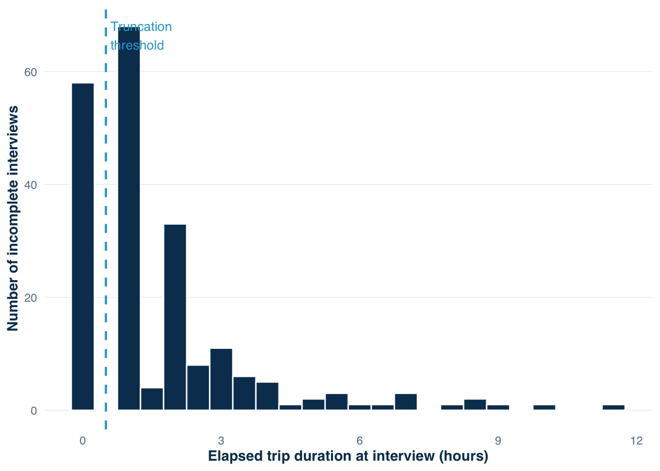
Of the 210 incomplete trips, 58 (27.6%) recorded elapsed durations below 0.5 hours. These short contacts — some as brief as 6 minutes — are precisely the records that inflate MOR variance. They are excluded from the Hoenig-recommended estimator.
Now compute both ROM and MOR, with and without truncation:
Code
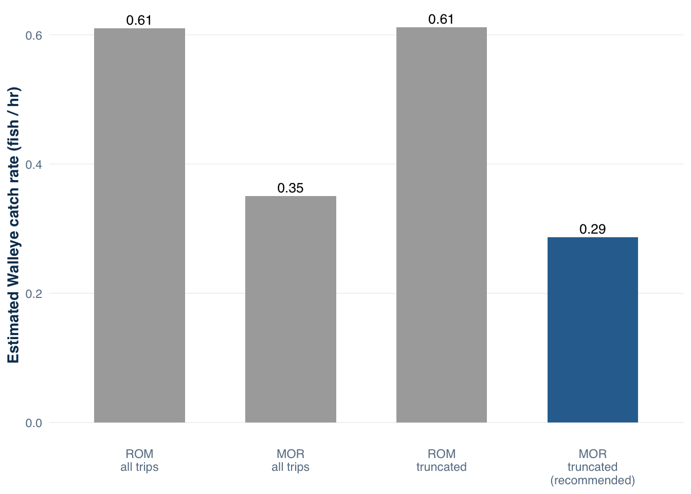
# All incomplete trips — no truncationrom_all <-sum(walleye_incomplete$walleye) /sum(walleye_incomplete$hours_fished)mor_all <-mean(walleye_incomplete$walleye / walleye_incomplete$hours_fished)# After truncation: exclude trips < 0.5 hours (Hoenig et al. 1997)walleye_trunc <- walleye_incomplete |>filter(hours_fished >=0.5)rom_trunc <-sum(walleye_trunc$walleye) /sum(walleye_trunc$hours_fished)mor_trunc <-mean(walleye_trunc$walleye / walleye_trunc$hours_fished)tibble(estimator =c("ROM — all trips", "MOR — all trips","ROM — truncated", "MOR — truncated (recommended)"),n_interviews =c(nrow(walleye_incomplete), nrow(walleye_incomplete),nrow(walleye_trunc), nrow(walleye_trunc)),rate =round(c(rom_all, mor_all, rom_trunc, mor_trunc), 4))
# A tibble: 4 × 3
  estimator                     n_interviews  rate
  <chr>                                <int> <dbl>
1 ROM — all trips                        210 0.610
2 MOR — all trips                        210 0.350
3 ROM — truncated                        152 0.612
4 MOR — truncated (recommended)          152 0.286
Figure 10.2: Walleye catch rate estimates under four estimator-sample combinations at Harlan Reservoir, 2022. ROM applied to all incomplete trips (top left) is the most common error: it overestimates catch rate because the denominator (elapsed hours) underrepresents true completed trip effort. MOR with truncation (bottom right) is the Hoenig et al. (1997) recommendation: it has the correct expectation and finite variance after short trips are removed.
The discrepancy between ROM (0.61 fish/hour) and MOR with truncation (0.29 fish/hour) is large — more than two-to-one. The gap has a structural explanation: ROM for incomplete trips gives disproportionate weight to high catch-rate observations in the denominator, while MOR averages individual rates and the truncation removes the most extreme observations. Neither estimate is “right” in an absolute sense; what matters is which estimator correctly targets the population quantity of interest given the incomplete-trip observation structure.
For comparison, the completed-trip total Walleye CPUE (harvest + release) using ROM is approximately 0.91 fish/hour — higher than both incomplete-trip estimators. This is not the harvest-only rate from Chapter 4 (which was 0.082 fish/hour; Harlan Walleye are predominantly catch-and-release, with 1,699 fish released versus 200 harvested). The ordering — completed-trip total CPUE (0.91) > ROM-all incomplete (0.61) > MOR-trunc (0.29) — is consistent with length-of-stay bias: shorter trips dominate the incomplete interview record and are less likely to represent the productive, fish-retaining sessions that make up a larger share of completed-trip fishing time.
The truncation decision
The 30-minute cutoff recommended by Hoenig et al. (1997) is a practical rule, not a mathematical requirement. It was chosen based on simulation studies showing that mean squared error decreased sharply when trips below 30–60 minutes were excluded, then leveled off for longer thresholds. Shorter thresholds (15 minutes) leave high-variance observations in the sample; longer thresholds (60 minutes) discard more data than necessary and can introduce truncation bias if the excluded trips are systematically different in catch rate from the retained trips.
In practice, the analyst should examine the trip duration distribution before settling on a threshold:
Code
ggplot(walleye_incomplete, aes(x = hours_fished)) +geom_histogram(binwidth =0.5, fill =creel_palette()["primary"], color ="white") +geom_vline(xintercept =0.5, linetype ="dashed", linewidth =0.8,color =creel_palette()["accent"]) +annotate("text", x =0.6, y =Inf, label ="Truncation\nthreshold",hjust =0, vjust =1.5, size =3.5,color =creel_palette()["accent"]) +labs(x ="Elapsed trip duration at interview (hours)",y ="Number of incomplete interviews" ) +theme_creel()
Figure 10.3: Distribution of elapsed trip durations for incomplete interviews at Harlan Reservoir, 2022. The vertical dashed line marks the 0.5-hour truncation threshold recommended by Hoenig et al. (1997). Trips to the left of this line are excluded from the mean-of-ratios catch rate calculation.
The spike at the left edge of the distribution reflects contacts made very early in a shift — sometimes within minutes of an angler launching. These observations contain little information about the trip’s eventual catch rate and introduce extreme per-unit-effort values that destabilize the MOR estimator.
10.8 Variance of the mean-of-ratios estimator
Hoenig et al. (1997) showed that the mean-of-ratios estimator has infinite variance when short trips are included — meaning the expected squared deviation from the true value is unbounded. Truncating short trips renders MOR variance finite and estimable from the data.
After truncation, the variance of MOR is estimated by the ordinary sample variance of the individual catch rates r_j = c_j / l_j:
n (after truncation): 152
 MOR estimate: 0.2865 fish/hr
 SD of individual rates: 0.9205
 SE: 0.0747
 CV: 26.1 %
The coefficient of variation of approximately 26% is high by conventional precision standards (CV ≤ 20% is often cited as a target). This reflects genuine overdispersion in the Walleye catch rate: most anglers catch nothing during the interviewed interval, a few catch many fish, and the short-trip truncation does not fully remove the leverage of occasional high catch-rate contacts. Improving precision would require a larger sample of incomplete interviews, temporal stratification of interviews, or supplementary information from completed-trip contacts.
Variance can also be estimated using a Taylor-series expansion that accounts for the covariance between the count-based effort estimate and the interview-based catch rate. tidycreel implements Taylor variance for both ROM and MOR estimators through estimate_catch_rate():
Code
est <-estimate_catch_rate(design = harlan_design_final,estimator ="mortr",truncate_at =0.5)
ℹ Using incomplete trips for CPUE estimation
  (n=210, 35% of 600 interviews)
Warning: ! MOR estimator for incomplete trips. Complete trips preferred.
ℹ Using MOR with n=210 incomplete of 210 total interviews.
ℹ Incomplete trips may have length-of-stay bias (Pollock et al.).
ℹ Validate incomplete estimates with `validate_incomplete_trips()` (Phase 19).
Warning: ! MOR truncation: 58 trips excluded (27.6%)
ℹ Trips < 0.5 hours excluded to prevent unstable variance
! High truncation rate may indicate data quality issues
ℹ Consider reviewing trip duration data for errors
Code
est
── DIAGNOSTIC: MOR Estimator (Incomplete Trips) ────────────────────────────────
! Complete trips preferred for CPUE estimation.
Uses incomplete trip interviews only (152 trips).
Truncation: 58 trips excluded (< 0.5 hours)
Validate with `validate_incomplete_trips()` before use (Phase 19).


── Creel Survey Estimates ──────────────────────────────────────────────────────
Method: Truncated Mean-of-Ratios CPUE
Variance: Taylor linearization
Confidence level: 95%
Unit: fish/angler-hour

# A tibble: 1 × 5
  estimate    se ci_lower ci_upper     n
     <dbl> <dbl>    <dbl>    <dbl> <int>
1    0.792 0.166    0.466     1.12   152
The truncate_at argument applies the 0.5-hour threshold automatically. The estimator = "mortr" argument selects the truncated mean-of-ratios formula rather than the ratio-of-means default. The overall CPUE of 0.792 fish/hr from the Taylor-variance estimator is slightly higher than the manually computed MOR of 0.29 fish/hr for Walleye alone, because here it uses the aggregated harvest total across all species rather than Walleye-only counts.
10.9 Diagnosing incomplete trips with validate_incomplete_trips
Before computing catch rates from incomplete interviews, tidycreel provides a diagnostic function that checks the incomplete-trip record for issues that would bias the MOR estimate:
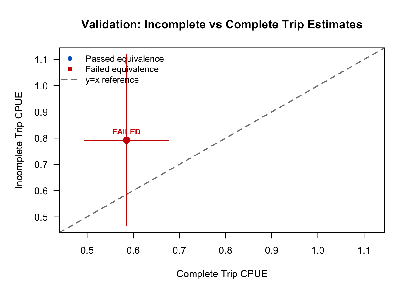
── TOST Equivalence Validation Results ─────────────────────────────────────────
Threshold: ±20% of complete trip estimate
✖ Validation FAILED

Recommendation: Validation failed: Use complete trips only (estimates not
statistically equivalent)


── Overall Test ──

Complete trips: n = 390, CPUE = 0.585
Incomplete trips: n = 152, CPUE = 0.792
Difference: -0.207
Equivalence bounds: [-0.117, 0.117]
TOST p-values: p_lower = 0.6981, p_upper = 0.0313
✖ Overall equivalence: FAILED
The function runs a two one-sided tests (TOST) equivalence procedure that compares the CPUE of complete and incomplete trips. If the two groups produce catch rates that are statistically indistinguishable within a ±20% equivalence band, the validation passes. If the gap between complete and incomplete trip CPUE falls outside that band, validation fails and the recommendation is to use complete trips only.
At Harlan, validation fails. Incomplete trip CPUE (0.792 fish/hr) exceeds complete trip CPUE (0.585 fish/hr) by more than the 20% equivalence threshold. This pattern is consistent with length-of-stay bias operating in the expected direction: anglers who had already caught fish when contacted were more likely to continue fishing, inflating mid-trip catch rates relative to completed-trip rates. The failed validation does not invalidate the roving data; it confirms that the two trip types capture different moments in the angling process and should not be pooled without appropriate estimator selection.
Running validate_incomplete_trips() before computing estimates is especially important in programs that combine access-point and roving contacts in a single dataset, as is common when technicians collect both completed and incomplete interviews on the same day.
10.10 Total catch from roving data
Total catch from a roving survey is the product of estimated effort and estimated catch rate, following the same two-component structure as the access-point design but with different estimators for each component:
where \hat{E} is the effort estimate from instantaneous or progressive counts (in angler-hours) and \hat{R}_{\text{MOR}} is the mean-of-ratios catch rate from the truncated incomplete interview sample.
For a single sampled period, the calculation is direct:
Code
# Effort for September 2, 2022, morning period (from earlier calculation)effort_sep2_period1 <-mean( harlan_counts |>filter(date ==as.Date("2022-09-02"), period ==1) |>mutate(total = angler_count) |>pull(total)) * shift_hours["1"]# MOR Walleye catch rate (computed above)walleye_mor <-mean(walleye_trunc$walleye / walleye_trunc$hours_fished)# Period total catch estimatetotal_walleye_period <- effort_sep2_period1 * walleye_morcat("Effort (period):", round(effort_sep2_period1, 1), "angler-hours\n","Walleye MOR:", round(walleye_mor, 4), "fish/hr\n","Estimated Walleye catch:", round(total_walleye_period, 1), "fish\n")
This single-period estimate illustrates the scale of the calculation. Seasonal totals require summing across all sampled periods, stratified by day type and period, and expanding to the full season day count — the same stratification logic applied to effort in Chapter 4.
The variance of the total catch estimate propagates from both the effort variance and the catch rate variance. Under the delta method:
In practice, the catch rate variance often dominates when the interview sample is small or the species is patchily distributed. The effort variance dominates when the count sample is small relative to day-to-day fluctuation in angler activity. For Walleye at Harlan, the large CV on the MOR estimate (26%) suggests that catch rate uncertainty will be the primary driver of total catch variance.
10.11 Preparing interview data for roving analysis
The prep_interviews_trips() function in tidycreel standardizes interview data for downstream analysis, including roving designs. The trip_status argument is the key field that tells tidycreel which interviews are complete and which are incomplete:
Code
# Standardize interview records with explicit trip_status fieldinterviews_prepped <-prep_interviews_trips(data = raw_interview_data,date = survey_date,interview_uid = interview_id,effort_hours = hours_fished,trip_status = trip_status, # "complete" or "incomplete"strata =c(day_type, period))
When trip_status = "incomplete", downstream functions in tidycreel automatically route the interview to the MOR estimator and apply the truncation. When trip_status = "complete", the same data feed the ROM estimator. Programs that combine both completed and incomplete interviews in a single dataset — as Harlan does — can process all interviews through prep_interviews_trips() once and let estimate_catch_rate() apply the correct estimator to each subset.
tidycreel also provides summarize_trips() for a quick tabulation of the interview sample by status, species, and period:
Code
summarize_trips(harlan_design_final)
Trip Status Summary

Total interviews: 600
  Complete:   390 (65%)
  Incomplete: 210 (35%)

Duration (hours) by status:
  complete: min=0.1, median=4.55, mean=4.74, max=13.82
  incomplete: min=0.1, median=1.06, mean=1.71, max=11.44
The output reports total interview counts, the completed/incomplete split, and summary statistics for elapsed duration by trip status. The 4.74-hour mean for completed trips and 1.71-hour mean for incomplete trips match the manual calculation from the length-of-stay comparison earlier in this chapter, confirming that the design object carries the same data used in the worked examples and that the trip-status routing is correct before estimation proceeds.
10.12 When to use roving surveys
Table 10.1 summarizes the conditions that favor roving versus access-point designs. In practice, the choice is rarely binary: many surveys combine both methods, using access-point interviews for boat anglers at ramps and roving contacts for bank anglers along diffuse shoreline.
Table 10.1: Design choice between access-point and roving creel surveys.
Condition
Access-point
Roving
Finite, enumerable entry/exit points
Preferred
Unnecessary
Diffuse shoreline or bank access
Poor coverage
Required
Private docks and informal landings
Missed entirely
Countable
River reach spanning many access sites
Impractical to staff
Natural fit
Completed-trip data needed for ROM
Provides directly
Requires follow-up
Site-specific spatial resolution needed
High per site
High per route segment
Recall bias for released catch
Some risk
Minimal (interview during trip)
Field logistics complexity
Moderate
Higher
Cost per interview
Lower
Higher to much higher
Incomplete-trip bias risk
None
Inherent
Pollock et al. (1994, Ch. 15) note that the roving design — roving counts paired with roving interviews — “despite some serious drawbacks, is probably the most widely used on-site creel survey design.” Its ubiquity reflects the reality that most productive fisheries in North America do not funnel through a compact access network. Rivers, reservoirs with dispersed access, natural lakes with extensive shoreline, and coastal fisheries all require some form of roving contact if bank and shoreline anglers are to be sampled.
The serious drawbacks Pollock et al. identify are real. Effort estimates from instantaneous counts can have severe negative bias when count times are not randomized or when clerks systematically avoid high-pressure areas. Incomplete-trip interviews require the analyst to choose the correct estimator and apply the truncation rule; the wrong choice produces biased catch rate estimates that persist undetected through the full seasonal expansion. And the length-of-stay bias — the oversampling of long trips — cannot be fully corrected without additional data on the distribution of completed trip lengths, which roving surveys cannot supply.
Understanding these constraints is not an argument against roving surveys. It is an argument for designing them carefully, executing them consistently, and analyzing them with estimators that match the observation structure. The tools in tidycreel — validate_incomplete_trips(), estimate_catch_rate() with estimator = "mean-of-ratios", and prep_interviews_trips() — are designed to make that match automatic and auditable.
10.13tidycreel support
Implemented for roving designs:
prep_interviews_trips() — standardizes interview data; trip_status field routes complete vs. incomplete records to correct estimators
estimate_catch_rate(estimator = "mean-of-ratios", truncate_at = 0.5) — MOR with Hoenig truncation for incomplete trips
validate_incomplete_trips() — diagnostic checks on roving interview sample quality
summarize_trips() — tabulation of interview sample by trip status and stratum
compute_effort() — effort from interview timestamps (trip start to interview time); used inside prep_interviews_trips()
audit_strata() — checks that count and interview strata are compatible before estimation
Progressive count effort estimation — fully supported via add_counts(count_type = "progressive", circuit_time = 2, period_length_col = shift_hours), where circuit_time is the route traversal time τ in hours and period_length_col names the column holding shift duration T_d; κ = T_d / τ is computed internally following the Hoenig et al. (1993) estimator
generate_progressive_start() — schedules randomised circuit start times (discrete or wraparound strategy) per Hoenig et al. (1993); avoids the U[0, T − τ] mid-day bias error common in manual scheduling
Partially supported:
Combined access-point and roving designs — prep_interviews_trips() handles both in a single call; stratum-specific estimator selection is manual in the current version
Manual or conceptual:
Correcting length-of-stay bias — no correction is available; bias direction and magnitude require knowledge of the completed trip distribution
Nonstationary catch rate diagnosis — the analyst must compare incomplete-trip MOR to completed-trip ROM; systematic differences suggest nonstationarity that biases both estimators
Hybrid designs combining roving counts with access-point interviews — supported analytically but requires explicit stratum construction
10.14 Takeaway
Roving surveys extend creel sampling to fisheries that access-point designs cannot reach. The price of that flexibility is methodological discipline: effort must come from counts, catch rate must come from mid-trip interviews using the mean-of-ratios estimator, and trips shorter than 30 minutes should be excluded to keep variance manageable. The length-of-stay bias that is intrinsic to roving contact cannot be corrected from within the survey data, but its direction and approximate magnitude can be assessed by comparing mean elapsed interview time to the mean completed-trip duration from any completed-trip contacts available in the same program.
At Harlan, the 210 incomplete interviews produced a Walleye MOR of approximately 0.29 fish/hour after truncation — substantially lower than the ROM applied naively to all incomplete trips (0.61 fish/hour) and lower than the completed-trip total Walleye CPUE using ROM (0.91 fish/hour; harvest + release combined, not the harvest-only rate of 0.082 fish/hour reported in Chapter 4). The gap among those three numbers summarizes the main risks of misapplying estimators: the wrong formula does not produce a warning, it just produces a number that looks plausible and is wrong.
Hoenig, J. M., C. M. Jones, K. H. Pollock, D. S. Robson, and D. L. Wade. 1997. Calculation of catch rate and total catch in roving surveys of anglers. Biometrics 53(1):306–317.
Hoenig, J. M., D. S. Robson, C. M. Jones, and K. H. Pollock. 1993. Scheduling counts in the instantaneous and progressive count methods for estimating sportfishing effort. North American Journal of Fisheries Management 13(4):723–736.
Malvestuto, S. P., W. D. Davies, and W. L. Shelton. 1978. An evaluation of the roving creel survey with nonuniform probability sampling. Transactions of the American Fisheries Society 107(2):255–262.
Pierce, R. B., and A. G. Bindman. 1994. Management briefs: Comparison of absolute fishing effort and hourly instantaneous angler counts in a small lake. North American Journal of Fisheries Management 14(2):447–448.
Pollock, K. H., C. M. Jones, and T. L. Brown. 1994. Angler survey methods and their applications in fisheries management. American Fisheries Society, Bethesda, Maryland.