creel survey, fisheries, design-based inference, R, tidycreel, Quarto
9.1 Why access-point surveys work
Access-point creel surveys are historically the most common design in inland fisheries management (Pollock et al. 1994). The logic behind them is straightforward: if anglers must pass through a finite set of access points to reach and leave a fishery, a technician stationed at those points can count who is present and interview who has finished fishing. Two types of observations — counts and interviews — answer two related but distinct questions: how many angler-hours occurred, and at what rate were fish caught per angler-hour.
What makes access-point surveys tractable is that the sampling frame is physically visible. Boat ramps, parking lots, dock areas, and piers are defined locations that can be enumerated before the survey starts. A technician knows when they are at a covered point and when they are not. This visibility makes the coverage assumptions explicit in a way that purely probabilistic designs cannot match.
The design is not without limitations. Access networks rarely cover an entire fishery. Shore anglers who reach the water through unimproved trails, anglers using private docks, and ice anglers accessing frozen surfaces through locations not included in the ramp network may all be missed. Whether those exclusions matter depends on the management question and the share of total effort they represent.
This chapter works through the access-point design from first principles: how the frame is defined, how counts translate to effort estimates, how completed-trip interviews produce catch rates through the ratio-of-means estimator, and where the design is vulnerable to bias. The example throughout is Harlan Reservoir, where the access network is simplified to a primary ramp and a secondary bank-fishing area.
9.2 Constructing the access-point frame
The access-point frame is the set of spatial and temporal opportunities that define the survey’s population of inference. As Pope et al. ((in press)) emphasize, a frame that fails to enumerate real fishing activity produces estimates that undercount the true total, regardless of how carefully the covered access points are sampled.
A well-constructed frame answers four questions explicitly:
Which access points are included, and which are excluded?
What temporal domain does the survey cover — which days, which hours, which seasons?
What angler types are covered at each access point?
What is the procedure for drawing access points and time periods into the sample?
In practice, frame construction begins with a site inventory. Every location where anglers routinely enter or exit the fishery is catalogued. Common omissions include informal shore-access points reached through adjacent private land, wading access from road bridges, and seasonal-use sites that are active only during ice or low-water conditions. Including a site in the frame does not mean it will be sampled on every visit; it means the site has a known, nonzero probability of being selected.
At Harlan Reservoir, the frame covers the primary boat ramp, a secondary bank-fishing area, and the connecting access road. Section 0 in the data represents the combined access network as a single spatial unit. In a design with multiple distinct access points — a bus-route design, treated in the next section — each site would carry its own inclusion probability.
Once spatial coverage is settled, the temporal frame must be defined. For Harlan, the frame spans 211 days from April through October 2022, divided into two strata — weekdays (Monday–Friday) and weekends (Saturday–Sunday plus holidays). Of those 211 days, 116 were sampled. Each sampled day was assigned to one of two shift periods: a morning period (roughly 6 a.m. to 2 p.m.) or an afternoon period (roughly 2 p.m. to 8 p.m.).
9.3 The bus-route design
When a fishery has multiple access points spread across a large area, a single technician cannot cover them simultaneously. The bus-route design solves this logistically: the technician follows a circuit, visiting each access point in sequence and spending a defined amount of time at each stop. The name comes from the analogy of a bus that visits a sequence of stops on a route.
Pope et al. ((in press)) describe the bus-route design as the primary multi-site variant of the access-point survey. The circuit is planned in advance: each stop is included in the route, and the time allocated to each stop — the wait timew_j — is specified before the survey begins. The technician counts and interviews at each stop for the allocated time, then moves to the next.
Effort estimation on a bus route
The effort formula for a bus-route design differs from the single-site formula. Let T be the total circuit length in hours, w_j be the wait time at stop j, and e_{jk} be the time that vehicle (or boat trailer) k is parked at stop j while the technician is present. The estimated effort on the circuit is:
\hat{E} = T \sum_{j=1}^{J} \frac{1}{w_j} \sum_{k=1}^{m_j} e_{jk}
Each vehicle’s contribution is scaled by 1/w_j — the inverse of the time the technician spent at that stop. A vehicle present for the full wait time (e_{jk} = w_j) contributes T angler-hours to the total. A vehicle that arrived just as the technician was leaving (e_{jk} \approx 0) contributes almost nothing.
The logic reflects the same inclusion-probability principle from Chapter 3. A vehicle parked for a long time had a higher probability of being observed on any given visit; scaling by 1/w_j corrects for the differential observation probability across stops with different wait times.
Read as plain language, the formula says that a stop with longer parking times contributes less per observed vehicle because the observer had more chances to see it. That is the same design idea that turns a count of anglers into a time-based estimate of effort.
Scheduling the route
The tidycreel package supports bus-route designs through generate_bus_schedule(), which randomizes the circuit order and assigns visit windows to each stop within the daily sampling period:
Randomizing the circuit order is important. If the technician always visits the main ramp first, count times at the main ramp are always early in the day — potentially during peak or off-peak periods in a non-representative way. A randomized visit order distributes the technician’s presence more evenly across the day.
When to use bus-route versus single-site
Table 9.1: Design choice between single-site and bus-route access-point designs.
Condition
Single-site
Bus-route
Dominant access point covers most use
Preferred
Not needed
Multiple sites with distinct populations
Poor coverage
Required
Spatial disaggregation is a goal
Cannot support
Supports
Interview density per stop matters most
Higher
Lower
Logistical cost is a constraint
Lower
Higher
The trade-off is interview density within a stop versus spatial coverage across stops. A technician who spends 45 minutes at each of four stops cannot accumulate the same within-stop interview count as a technician stationed at one location for three hours. When the management question requires reservoir-wide totals rather than site-specific comparisons, the single-site design serving the dominant access point may be sufficient.
9.4 The two-component structure
Every access-point survey produces two types of field records that serve complementary roles.
Counts answer the question: how many anglers were present at the access point during a defined time? Counts are typically instantaneous — a technician records the number of anglers or boats observed at a specific moment. Repeating counts at multiple times within a shift allows the mean within-period count to be estimated. That mean count, multiplied by the shift duration, converts to angler-hours of effort.
Interviews answer the question: what did those anglers catch, and how long did they fish? A completed-trip interview captures the full trip record — hours fished, species caught, fish harvested and released, and angler characteristics. When the interview occurs as a party departs the access point, the information reflects the entirety of their time on the water.
Neither data type is sufficient alone. Counts yield an effort total with no catch information. Interviews yield trip-level catch rates with no expansion factor. The estimation step combines both: the catch rate from interviews is applied to the effort total from counts.
Code
# Counts: two count times per shift period, per sampled dayharlan_counts |>group_by(date, period) |>summarise(n_counts =n(),total_anglers =sum(angler_count),.groups ="drop" ) |>group_by(period) |>summarise(n_shifts =n(),mean_total =round(mean(total_anglers), 1),sd_total =round(sd(total_anglers), 1),.groups ="drop" )
harlan_interviews |>count(trip_status) |>mutate(pct =round(100* n /sum(n), 1))
# A tibble: 2 × 3
  trip_status     n   pct
  <chr>       <int> <dbl>
1 complete      390    65
2 incomplete    210    35
The proportion of complete versus incomplete trips affects which estimator is appropriate for catch rates. This distinction is central to the access-point design logic and is addressed in full after the ratio-of-means section.
9.5 Effort estimation from counts
The standard effort estimator for an access-point survey converts instantaneous angler counts into angler-hours. The notation follows Bernard et al. ((1998)).
Let r_i be the number of count times within sampled period i, and let x_{it} be the count of anglers at count time t within that period. The mean count for period i is
If the period spans T hours (the shift duration), the estimated angler-hours for that period is
\hat{E}_i = T \cdot \bar{x}_i.
This formula rests on a strong assumption: angler density at the count times is representative of angler density throughout the shift. That assumption is most defensible when count times are drawn randomly or systematically within the shift window, and least defensible when counts are scheduled at times that are systematically more or less active than the rest of the shift.
For a seasonal total, the period-level estimates are expanded to the full frame using the same Horvitz-Thompson logic from Chapter 3. If d periods were sampled from a frame of D periods in stratum h:
where N_h is the number of periods in the frame for stratum h and n_h is the number sampled.
A worked example: Harlan Reservoir, September 2, 2022
The arithmetic is easier to follow through a specific field day. On September 2, 2022 — a weekday morning shift at Harlan — a technician made two instantaneous counts during period 1 (the morning shift, T = 8 hours):
Table 9.2: Instantaneous counts at Harlan Reservoir, September 2 morning shift.
Count time
Bank anglers
Boat anglers
Total
09:00
0
38
38
11:15
0
45
45
With r_i = 2 count times and observations x_{i1} = 38, x_{i2} = 45:
This single shift contributes 332 angler-hours to the seasonal total. In the HT expansion, that estimate is multiplied by its stratum expansion factor. The weekday stratum has N_h = 150 days in the frame and n_h = 83 sampled periods, giving w = N_h / n_h = 150 / 83 \approx 1.81. The weighted contribution of this one day is 332 \times 1.81 \approx 601 angler-hours.
The implicit assumption is that the 41.5 anglers observed at 9:00 and 11:15 are representative of angler density throughout the full 8-hour shift — including the early morning before 9:00 and the late morning after 11:15. Whether that assumption holds depends on how count times were chosen. Random or systematic spacing within the shift window makes this defensible. Counts bunched near the expected peak of activity inflate the mean count and bias \hat{E}_i upward.
Code
# Period length in hours for each shift (morning ≈ 8 h, afternoon ≈ 6 h)shift_hours <-c("1"=8, "2"=6)# Step 1: mean count per period-day, then multiply by shift durationdaily_effort <- harlan_counts |>group_by(date, day_type, period) |>summarise(n_counts =n(),mean_total =mean(angler_count),.groups ="drop" ) |>mutate(T_hours = shift_hours[as.character(period)],effort_hat = mean_total * T_hours )daily_effort |>group_by(day_type, period) |>summarise(n_shifts =n(),mean_effort =round(mean(effort_hat), 1),sd_effort =round(sd(effort_hat), 1),.groups ="drop" )
The weekday and weekend strata produce separate effort estimates that are then summed. The finite population correction shrinks the variance contribution from strata where the sampling fraction is high.
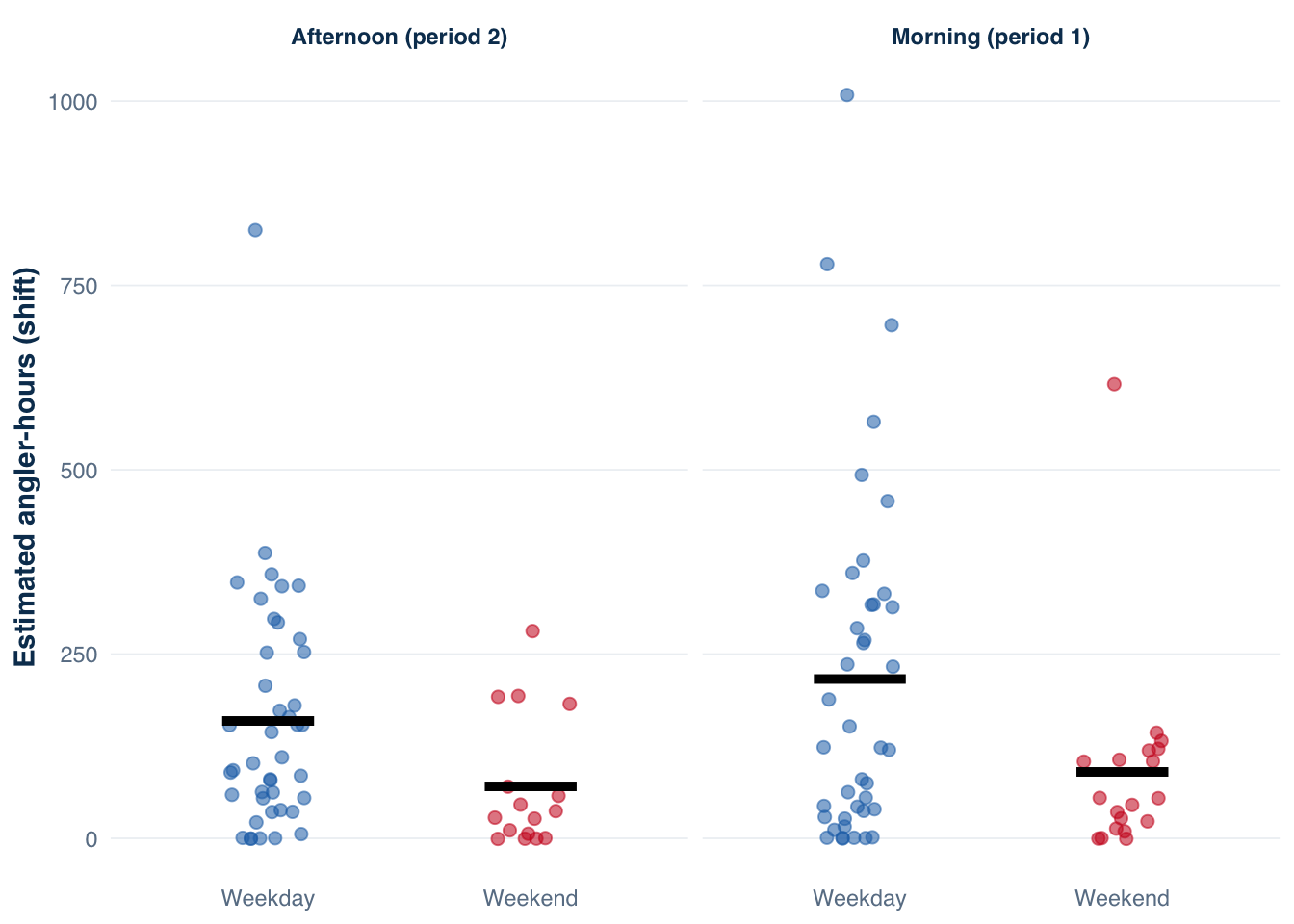
Figure 9.1: Distribution of estimated angler-hours per shift period at Harlan Reservoir by day type and period. Each point is one sampled shift. Morning shifts (period 1) yield higher effort than afternoon shifts in both strata. Weekday shifts produce substantially higher mean effort than weekend shifts, with greater absolute spread as well.
9.6 Completed-trip interviews and the selection advantage
Access-point surveys interview anglers at departure — a design choice that carries important statistical consequences.
When a party is interviewed as it leaves, the interview captures the entire trip: all the hours fished, all the fish caught, all the fish released. No extrapolation is needed because the record is already complete. Recall bias is minimal because the activity just ended. And the interviewer can inspect the catch directly rather than relying entirely on self-report.
Compare this with a survey that intercepts anglers mid-trip. A party interrupted at midday has fished some fraction of their eventual trip. If the interview uses the hours-so-far as the denominator in a catch-rate calculation, the result can be biased in ways that are difficult to quantify. Short-trip parties are more likely to have completed their trip when the interviewer arrives; long-trip parties are more likely to still be fishing. This creates a selection probability that depends on trip length — and trip length is correlated with what anglers catch.
The completed-trip feature of access-point surveys breaks that correlation. At departure, every party — short-trip or long-trip — has the same probability of being intercepted, assuming the technician is present and interviews all departing parties. The selection probability does not depend on trip duration. That is why the ratio-of-means is the right estimator here.
Put another way, the access-point interview sees the trip only after it is finished, so the numerator and denominator describe the same completed event. That is what makes the ratio meaningful without extra correction.
Code
# Complete vs incomplete trip breakdown by day typeharlan_interviews |>group_by(day_type, trip_status) |>summarise(n =n(), .groups ="drop") |>pivot_wider(names_from = trip_status, values_from = n, values_fill =0) |>mutate(pct_complete =round(100* complete / (complete + incomplete), 1))
Some parties are recorded as incomplete — they were intercepted before finishing their trip, or their trip status was ambiguous at interview time. At Harlan, roughly 35% of interviews are incomplete. This is a large fraction that requires explicit handling; the consequences are examined in the section on incomplete trips and catch-rate bias after the estimator is established.
9.7 The ratio-of-means estimator
Catch rate — fish caught per angler-hour — is the central currency of creel survey analysis. It links the effort estimate (angler-hours from counts) to a total catch estimate. The ratio-of-means (ROM) estimator is the standard approach for completed-trip access-point surveys.
Why ratio-of-means, not mean-of-ratios
Two estimators are sometimes proposed for catch rate from interview data.
The mean-of-ratios computes the catch rate for each party (c_k / e_k) and averages across parties:
The mean-of-ratios approach has two practical deficiencies. First, parties with very short trips, where (e_k \approx 0), can produce extreme or undefined ratios that dominate the average. Second, because each party receives equal weight, a 30-minute trip contributes as much to the estimate as an 8-hour trip. This makes the estimator sensitive to the distribution of trip lengths in the sample, whereas a ratio-of-means estimator weights observations implicitly by fishing effort and is therefore less affected by short, low-effort trips.
The ratio-of-means avoids both problems. Short trips contribute proportionally small weight to the denominator. Parties with zero catch but nonzero effort do not cause computational problems. And the estimator is equivalent to a weighted average of individual catch rates, with each party weighted by its contribution to total effort — which is the natural weighting for a rate defined per unit of effort (Hoenig et al. 1997).
The practical interpretation is straightforward: ROM answers the question, “How many fish were caught per hour across all finished trips?” It does not average every party equally; it pools their effort first and then forms the rate.
For a completed-trip access-point survey, Hoenig et al. ((1997)) show that the ROM estimator is less biased than the mean-of-ratios, particularly when trip length is correlated with catch. The intuition is that parties who catch fish quickly may end trips early, and the ratio-of-means down-weights their contribution in proportion to their shorter trips.
Let m be the number of interviewed parties with completed trips, c_k be the catch (or harvest) by party k, and e_k be the hours fished by party k. The ratio-of-means catch rate is
The total catch estimate combines this rate with the effort estimate:
\hat{C} = \hat{E} \cdot \hat{R}
where \hat{E} is the seasonal effort estimate from counts. The product \hat{E} \cdot \hat{R} is the fundamental identity of creel survey estimation: effort (from counts) times catch rate (from interviews) equals total catch.
Table 9.4 summarizes the notation used in this chapter.
Table 9.4: Key notation for access-point creel survey estimation.
Symbol
Definition
r_i
Number of count times in period i
x_{it}
Angler count at time t within period i
\bar{x}_i
Mean count across count times in period i
T
Shift duration in hours
\hat{E}_i
Estimated angler-hours for period i (= T \bar{x}_i)
\hat{E}
Seasonal effort estimate (expanded from all periods)
m
Number of interviewed parties with completed trips
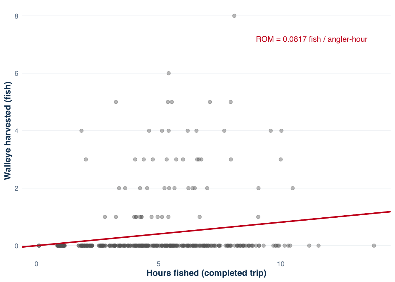
Figure 9.2: Walleye harvest versus hours fished per completed-trip party at Harlan Reservoir. The ratio-of-means estimator (red line slope) summarizes the catch rate using the pooled totals rather than a mean of individual ratios. Parties with long trips and zero harvest anchor the denominator without distorting the numerator, which is the desired behavior for a per-angler-hour rate.
9.8 Length-of-stay bias
The ratio-of-means estimator is appropriate for completed-trip interviews, but not necessarily for mid-trip intercepts. Understanding why requires the concept of length-of-stay bias, which Hoenig et al. ((1997)) analyzed formally.
The intuition is simple: when the interview happens at the end of the trip, every finished trip is eligible in the same way. When the interview happens in the middle, long trips are easier to catch than short trips, so the sample no longer reflects the trip population one-for-one.
Consider a survey that intercepts anglers at a random point during a period, rather than at departure. At that moment, who is most likely to be present? Anglers on long trips. A party fishing for ten hours has ten times the probability of being present at a random count time compared to a party that fished for one hour. If catch and trip length are correlated — which they typically are — this length-biased sampling systematically overrepresents productive anglers in the sample.
The bias flows through to the catch rate estimate. A sample enriched with long-trip, high-catch parties will produce inflated catch-rate estimates if the analysis does not correct for differential selection probabilities.
For a roving survey (Chapter 5), this length-of-stay bias must be explicitly corrected using methods that account for the duration of each party’s trip. The correction changes which estimator is appropriate: instead of the ratio-of-means from completed-trip totals, a roving survey requires an estimator that reweights each party by the inverse of their probability of selection, which is proportional to trip length (Hoenig et al. 1997).
An access-point survey with completed-trip interviews avoids this problem entirely. Every party that finishes a trip and exits through the access network has the same probability of being intercepted, regardless of how long they fished. The selection mechanism does not depend on trip duration. The ratio-of-means is therefore unbiased — no reweighting for trip length is necessary.
This is one of the principal statistical advantages of the access-point completed-trip design over roving designs. It comes at a logistical cost: the interviewer must wait at the access point for parties to complete their trips, which may mean long waits at low-use ramps.
9.9 Variance of the ratio-of-means
The ratio-of-means is a nonlinear function of two random variables (total catch and total effort). Exact variance calculation is not available in closed form, so the standard approach is a Taylor series (delta method) approximation.
Let \bar{c} = \frac{1}{m}\sum c_k and \bar{e} = \frac{1}{m}\sum e_k. The ratio \hat{R} = \bar{c}/\bar{e} has approximate variance
with s_c^2, s_e^2, and s_{ce} being the sample variance of catches, sample variance of efforts, and sample covariance of catch and effort across the m interviewed parties.
The full variance of the total catch estimate \hat{C} = \hat{E} \cdot \hat{R} must propagate uncertainty from both components. Using Goodman’s (1960) formula for the product of two independent random variables (Bernard et al. 1998):
In practice, the last term is small and sometimes omitted. The dominant contribution typically comes from \hat{V}(\hat{E}) — the between-day variability in effort — rather than from \hat{V}(\hat{R}). This parallels the finding in Chapter 3 that between-period variance drives most of the uncertainty in seasonal estimates.
cat("Variance from catch-rate uncertainty:",round(100* V_from_ROM / V_C, 1), "%\n")
Variance from catch-rate uncertainty: 81.2 %
The variance decomposition reveals which component limits precision. At Harlan, catch-rate uncertainty accounts for roughly 80% of the total variance in the Walleye harvest estimate. This is not unusual for a species with highly overdispersed catch — most parties catch zero Walleye, and the few parties that catch several drive nearly all the variability in \hat{R}. In this situation, more completed-trip interviews with Walleye records would improve precision more effectively than additional sampled days. The balance tips the other way for species with more consistent catch rates or when effort varies substantially day-to-day: then between-period effort variance dominates, and more sampled days is the efficient lever. The decomposition is the diagnostic tool for deciding which investment to make.
9.10 Incomplete trips and catch-rate bias
With 35% of Harlan interviews recorded as incomplete, the choice of whether to include them in the ratio-of-means matters — and the direction of bias is not always obvious.
An incomplete-trip party has hours-fished e_k^* that reflects only the portion of the trip completed at interview time, not the eventual trip total e_k. If catch also accrues at a constant rate throughout the trip, then c_k^* / e_k^* \approx c_k / e_k and including the incomplete record would not distort the ROM. In practice, this proportionality rarely holds for two reasons.
Suppression occurs when anglers who leave early have been less successful. A party that has not found fish after two hours may cut the trip short; their c_k^* / e_k^* is low. Including these parties pulls the catch rate down below what complete-trip parties would report.
Inflation occurs when anglers who leave early have been more successful. A party that reaches the bag limit after 90 minutes departs with a high c_k^* / e_k^*. Including these parties pushes the catch rate above the complete-trip estimate.
Which effect dominates depends on the species, the fishery, and the season. The only safe course is to examine the difference directly.
Code
# ROM from all trips pooled (including incomplete)all_trips <- harlan_interviews |>left_join(walleye_harvest, by ="interview_id") |>mutate(harvest =replace(harvest, is.na(harvest), 0L))rom_all <-sum(all_trips$harvest) /sum(all_trips$hours_fished)# Summary by trip statusall_trips |>group_by(trip_status) |>summarise(n =n(),total_fish =sum(harvest),total_hrs =round(sum(hours_fished), 1),mean_hours =round(mean(hours_fished), 2),ROM =round(sum(harvest) /sum(hours_fished), 4),.groups ="drop" )
The difference in ROM between complete and all trips is the empirical footprint of the incomplete-trip problem. At Harlan, incomplete parties show a Walleye harvest rate of 0.136 fish / angler-hour versus 0.082 for complete trips — a 67% difference. Pooling them inflates the combined ROM by roughly 11%. The pattern is consistent with inflation: anglers who reached their Walleye limit early departed before completing a full trip, and those short, high-catch sessions inflate the catch-rate numerator relative to the effort denominator. A large positive difference means incomplete parties have elevated catch rates. A large negative difference means they were less successful — short trips that ended early due to poor conditions or failure to find fish.
Whatever the direction, the complete-trip ROM is the defensible estimate. It corresponds to parties with known, equal selection probability at departure. The all-trips ROM conflates two different things: a catch rate from complete trips and a partial-trip rate from incomplete trips measured on different temporal scales. Chapter 11 covers formal tests for whether incomplete-trip ROM differs significantly from the complete-trip estimate, and the adjustment methods available when the sample of complete trips alone is too small to support reliable estimation.
9.11 Count frequency and effort precision
The variance of \hat{E}_i = T \bar{x}_i depends on how much angler density varies within the shift and on how many count times were taken. For r_i randomly placed count times within period i:
\hat{V}(\hat{E}_i) = T^2 \frac{s_{xi}^2}{r_i}
where s_{xi}^2 is the sample variance of the r_i counts within that period. Two implications follow directly.
First, more count times reduce within-period variance. Doubling r_i from 2 to 4 halves \hat{V}(\hat{E}_i). This is the within-period analog of sampling more days in the HT expansion.
Second, within-period variance has a floor set by between-period variance. No matter how many count times are taken within a shift, the uncertainty from day-to-day variability in fishing effort is unaffected. As shown in Chapter 3, between-period variance typically dominates the seasonal total variance. Additional counts per shift reduce a component of uncertainty that may already be small relative to the dominant source.
The practical implication: additional counts per shift help most when within-day angler density is highly variable — a ramp where fishing activity is concentrated in a narrow window and two standard counts might fall inside or outside that window by chance. When activity is more evenly distributed throughout the shift, additional counts add little precision.
Code
# Within-period variance per shift (two counts per period at Harlan)within_period <- harlan_counts |>group_by(date, day_type, period) |>summarise(r_i =n(),x_bar =mean(angler_count),s2_x =var(angler_count),.groups ="drop" ) |>mutate(T_h = shift_hours[as.character(period)],V_Ei = T_h^2* s2_x / r_i )# Contribution to total variance: within-period vs between-periodwithin_summary <- within_period |>group_by(day_type) |>summarise(mean_V_Ei =round(mean(V_Ei, na.rm =TRUE), 1),.groups ="drop" )within_summary |>inner_join(ht_effort |>select(day_type, V_hat), by ="day_type") |>mutate(within_pct =round(100* mean_V_Ei / V_hat, 2),between_pct =round(100- within_pct, 2) )
# Use weekday morning shifts (period 1) as referencewd_morning <- within_period |>filter(day_type =="weekday", period ==1)mean_s2x <-mean(wd_morning$s2_x, na.rm =TRUE)T_ref <-8between_SE <-sqrt(ht_effort$V_hat[ht_effort$day_type =="weekday"])count_curve <-tibble(r =1:12,V_Ei = T_ref^2* mean_s2x / r,SE_Ei =sqrt(V_Ei))ggplot(count_curve, aes(x = r, y = SE_Ei)) +geom_line(colour ="#2171b5", linewidth =1) +geom_point(colour ="#2171b5", size =2.5) +geom_hline(yintercept = between_SE,linetype ="dashed",colour ="#cb181d",linewidth =0.8 ) +annotate("text",x =9, y = between_SE *1.08,label ="Between-period SE",colour ="#cb181d", size =3.5, hjust =0 ) +geom_vline(xintercept =2, linetype ="dotted", colour ="#636363") +annotate("text",x =2.2, y =max(count_curve$SE_Ei) *0.93,label ="Harlan (r = 2)",colour ="#636363", size =3.2, hjust =0 ) +scale_x_continuous(breaks =1:12) +labs(x ="Number of count times per shift (r)",y ="Within-period SE of effort estimate (angler-hours)" ) +theme_creel()
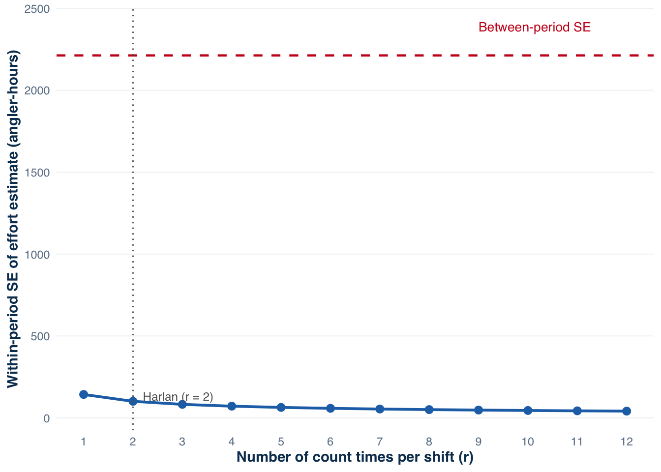
Figure 9.3: Simulated effect of increasing count frequency per shift on within-period standard error of the effort estimate, using observed within-day count variance from Harlan weekday morning shifts. The horizontal dashed line marks the between-period standard error, which is unaffected by count frequency. The current Harlan design uses r = 2 counts per shift (dotted vertical line). Adding counts past the crossover point — where within-period SE falls below between-period SE — produces negligible precision gains for the seasonal total.
At Harlan, between-period variance accounts for the large majority of the total variance in each stratum — confirmed by the table above. Moving from r = 2 to r = 4 would halve within-period SE but would not reduce the dominant between-period component. Investing the equivalent field time in additional sampled days is almost always more efficient.
9.12 Bias from unequal access-point sampling
Not all access-point designs have a single site. A reservoir with multiple boat ramps, a river with several access areas, or a lake with both boat and bank fishing locations presents a multi-site access-point design. When different sites receive different sampling intensity, unequal weighting must be applied to avoid spatial bias.
The bias mechanism is similar to the temporal bias from unequal day-type sampling discussed in Chapter 3. Suppose a reservoir has two boat ramps — a large main ramp that sees 80% of the angler traffic and a small secondary ramp that sees 20%. If the survey samples the main ramp on 90% of visits and the secondary ramp on 10%, each day’s sample overrepresents the main ramp. Estimates of total effort will be biased toward the main-ramp pattern. If catch rates differ between ramps — for example, because different access points serve different fishing zones — the catch estimate will also be biased.
The correction requires site-level inclusion probabilities: the probability that any given visit includes access point j. These probabilities are set at design time and must be documented for the weighting to work. If access points are sampled with unequal probability, the expansion weight for each site-visit is w_j = 1/\pi_j, where \pi_j is the inclusion probability for site j.
Malvestuto ((1996)) notes that undersampling low-use access points is a common design failure. The temptation is to concentrate effort where anglers are easy to find — high-use sites with good parking and reliable traffic. But low-use sites are not unimportant; they may serve specific angler populations (shore anglers, bank fishers, kayak anglers) whose behavior differs systematically from main-ramp users. Excluding or undersampling those sites introduces coverage bias that cannot be recovered from the interview data alone.
At Harlan, the counts data uses section = 0 throughout, indicating the design treated the reservoir’s access network as a single combined unit. This simplification is reasonable when the primary question is a reservoir-wide total. A study focused on spatially distinct angling populations — boat anglers versus bank anglers, for example — would require site-level stratification to avoid confounding access-type differences with temporal variation.
Code
# Angler types in the interview dataharlan_interviews |>filter(trip_status =="complete") |>count(angler_type, day_type) |>pivot_wider(names_from = day_type, values_from = n, values_fill =0)
# A tibble: 2 × 3
  angler_type weekday weekend
  <chr>         <int>   <int>
1 bank             52      19
2 boat            269      50
Code
# Walleye harvest rate by angler type — illustrates why site-level separation# matters if access points serve different populationstype_catch <- harlan_interviews |>filter(trip_status =="complete") |>left_join(walleye_harvest, by ="interview_id") |>mutate(harvest =replace(harvest, is.na(harvest), 0L))type_catch |>group_by(angler_type) |>summarise(n_parties =n(),ROM =round(sum(harvest) /sum(hours_fished), 4),mean_hours =round(mean(hours_fished), 2),.groups ="drop" )
# A tibble: 2 × 4
  angler_type n_parties    ROM mean_hours
  <chr>           <int>  <dbl>      <dbl>
1 bank               71 0.0067       2.09
2 boat              319 0.0882       5.33
The Walleye ROM differs sharply between boat and bank anglers. If boat and bank anglers access the fishery through separate physical locations, a design that samples only the boat ramp produces a catch-rate estimate that applies only to boat anglers. Reporting that estimate as a reservoir-wide catch rate implicitly excludes bank angling effort, and the exclusion is invisible in the estimate itself.
9.13tidycreel support
The tidycreel package implements the access-point estimation workflow through a design object that holds the schedule, counts, and interviews in a consistent structure. The full design-object pipeline is covered in Chapter 10; a brief preview here connects the manual calculations above to the package interface.
The entry point is creel_design(), which takes the survey calendar and defines the strata structure. Counts and interviews are added with add_counts() and add_interviews(). Once the design object is assembled, estimate_effort() and estimate_catch_rate() perform the HT expansion and ratio-of-means calculation internally, returning tidy output with estimates, standard errors, and confidence intervals.
The use_trips = "complete" argument restricts the catch-rate calculation to completed-trip records, enforcing the selection assumption that justifies the ratio-of-means. Incomplete trips can be included with adjustment using validate_incomplete_trips() before estimation, as described in Chapter 11.
Additional summarization functions — summarize_by_angler_type(), summarize_by_species_sought(), summarize_trips() — provide stratified breakdowns of the interview data that help identify whether catch rates differ systematically across subpopulations.
9.14 Common failure modes
Access-point surveys are vulnerable to a specific set of failures that coverage maps and interview counts do not make visible.
Targeting successful parties. Interviewing anglers at fish-cleaning stations, live wells, or while they handle their catch biases the sample toward successful trips. If successful parties agree to interview at higher rates than unsuccessful parties, catch-rate estimates are inflated. The correction is to intercept all departing parties randomly and record refusals — not to seek out anglers who look like they caught fish.
Pooling incomplete and complete trips without adjustment. Including incomplete-trip records in the ratio-of-means denominator as if they represented full trips introduces catch-rate bias in either direction depending on what drove early departure. Incomplete trips must be either excluded or adjusted before entering the calculation.
Treating access coverage as fishery coverage. An estimate of total angler-hours at the covered access network is not the same as an estimate of total angler-hours on the fishery. If 15% of fishing effort occurs through access points not in the frame, the estimate reflects 85% of the true total. The report should state which locations are covered and which are not, and whether the frame is expected to represent the full fishery.
Recording count period and interview period at different levels. Counts record anglers at specific times within a shift. Interviews record parties over the duration of a trip. If the data management system does not link counts and interviews to the same shift period, the effort-catch rate multiplication can apply the wrong count-based effort to the wrong set of interviews. The section and period columns in the Harlan data enforce this alignment; straying from a consistent period key in the field creates mismatches that are difficult to detect after the fact.
Scheduling counts around peak activity. Scheduling counts when the ramp is busiest produces a mean count higher than the true time-averaged density. \hat{E}_i = T \bar{x}_i is unbiased only when count times are drawn without regard to expected angler density. Stratifying count times to cover the full shift window, or drawing them randomly, guards against this form of upward bias.
9.15 Summary
Access-point creel surveys work because the spatial frame — the set of access points — is physically visible and enumerable. Technicians can count anglers at defined locations and interview departing parties, producing two compatible data streams: counts that estimate angler-hours and completed-trip interviews that estimate catch per angler-hour.
The key estimation identities are:
Effort per period: \hat{E}_i = T \cdot \bar{x}_i (mean count times shift duration)
Seasonal effort: HT expansion of period-level estimates across all sampled days
Variance: delta method for \hat{R}, Goodman’s formula for \hat{C}
The ratio-of-means is appropriate for completed-trip interviews because selection probability does not depend on trip length. This avoids the length-of-stay bias that requires correction in roving surveys. Incomplete trips must be excluded or adjusted before estimation — pooling them with complete trips introduces catch-rate bias whose direction depends on what drove early departure.
Between-period variance typically dominates the total variance budget. Increasing count frequency per shift reduces within-period variance but leaves the dominant component unchanged. More sampled days is almost always the more efficient precision investment. The design is as strong as its frame: access points not in the frame contribute nothing to the estimate regardless of how many anglers use them. That boundary should be stated explicitly in every report that uses access-point data.
Bernard, D. R., A. E. Bingham, and M. Alexandersdottir. 1998. Robust harvest estimates from on-site roving–access creel surveys. Transactions of the American Fisheries Society 127(3):481–495.
Hoenig, J. M., C. M. Jones, K. H. Pollock, D. S. Robson, and D. L. Wade. 1997. Calculation of catch rate and total catch in roving surveys of anglers. Biometrics 53(1):306–317.
Malvestuto, S. P. 1996. Sampling the recreational creel. Pages 591–623 in B. R. Murphy and D. W. Willis, editors. Fisheries techniques, 2nd edition. American Fisheries Society, Bethesda, Maryland.
Pollock, K. H., C. M. Jones, and T. L. Brown. 1994. Angler survey methods and their applications in fisheries management. American Fisheries Society, Bethesda, Maryland.
Pope, K. L., C. J. Chizinski, A. J. Lynch, and J. R. Post. in pressin press. Creel surveys.