creel survey, fisheries, design-based inference, R, tidycreel, Quarto
8.1 Purpose
Chapters 1–3 established the why — why creel surveys exist, what they estimate, and what makes the estimators statistically defensible. This chapter establishes the how before the theory goes deeper.
A complete tidycreel analysis has four steps: load the data, build a design object that encodes the survey structure, run the estimators, and summarize the results. This chapter walks through all four on the Harlan Reservoir dataset and produces defensible estimates of effort, harvest, and catch rate by the end. No theory not already in Chapters 1–3; just the pipeline running on real data.
If you want to see the complete sequence in one view, it fits in about forty lines:
The rest of this chapter works through each block in detail, explaining what each function expects and what its output means. Chapters 9–16 go deeper into every step.
8.2 The Harlan data
Four tables form the Harlan Reservoir dataset. They are linked by date and interview_id and must stay separate until the estimation step — collapsing them prematurely discards the information needed to apply the correct expansion weights. Chapter 9 covers the linked-table structure in detail; for now, looking at each table’s shape is enough.
# A tibble: 3 × 4
  interview_id species      catch_type n_fish
         <int> <chr>        <chr>       <int>
1            1 White Bass   released       11
2            1 White Bass   harvested      32
3            1 Yellow Perch released        1
The four tables represent four levels of resolution: which days were in the survey and which were sampled (schedule), instantaneous counts of anglers on sampled days (counts), one record per angler party per sampled day (interviews), and one record per species per catch type per party (catch). Every downstream estimate traces back to this structure.
Before building the design, confirm the tables are internally consistent:
── Creel Data Validation ───────────────────────────────────────────────────────
63 pass | 0 warn | 0 fail
── Table: counts ──
✔ reservoir
✔ type: class: character
✔ na_rate: 0 / 236 NA (0%)
✔ empty_strings: none
✔ date
✔ type: class: Date
✔ na_rate: 0 / 236 NA (0%)
✔ date_range: all within 1970-01-01 - 2100-12-31
✔ day_type
✔ type: class: character
✔ na_rate: 0 / 236 NA (0%)
✔ empty_strings: none
✔ period
✔ type: class: numeric
✔ na_rate: 0 / 236 NA (0%)
✔ negative_values: none
✔ section
✔ type: class: character
✔ na_rate: 0 / 236 NA (0%)
✔ empty_strings: none
✔ count_time
✔ type: class: character
✔ na_rate: 0 / 236 NA (0%)
✔ empty_strings: none
✔ bank_anglers
✔ type: class: integer
✔ na_rate: 0 / 236 NA (0%)
✔ negative_values: none
✔ angler_boats
✔ type: class: integer
✔ na_rate: 0 / 236 NA (0%)
✔ negative_values: none
✔ boat_anglers
✔ type: class: integer
✔ na_rate: 0 / 236 NA (0%)
✔ negative_values: none
── Table: interviews ──
✔ reservoir
✔ type: class: character
✔ na_rate: 0 / 600 NA (0%)
✔ empty_strings: none
✔ date
✔ type: class: Date
✔ na_rate: 0 / 600 NA (0%)
✔ date_range: all within 1970-01-01 - 2100-12-31
✔ day_type
✔ type: class: character
✔ na_rate: 0 / 600 NA (0%)
✔ empty_strings: none
✔ period
✔ type: class: numeric
✔ na_rate: 0 / 600 NA (0%)
✔ negative_values: none
✔ section
✔ type: class: character
✔ na_rate: 0 / 600 NA (0%)
✔ empty_strings: none
✔ interview_id
✔ type: class: integer
✔ na_rate: 0 / 600 NA (0%)
✔ negative_values: none
✔ party_id
✔ type: class: character
✔ na_rate: 0 / 600 NA (0%)
✔ empty_strings: none
✔ n_anglers
✔ type: class: numeric
✔ na_rate: 0 / 600 NA (0%)
✔ negative_values: none
✔ angler_type
✔ type: class: character
✔ na_rate: 0 / 600 NA (0%)
✔ empty_strings: none
✔ angler_method
✔ type: class: character
✔ na_rate: 0 / 600 NA (0%)
✔ empty_strings: none
✔ hours_fished
✔ type: class: numeric
✔ na_rate: 0 / 600 NA (0%)
✔ negative_values: none
✔ trip_status
✔ type: class: character
✔ na_rate: 0 / 600 NA (0%)
✔ empty_strings: none
A clean pass here means no column-type errors, no impossible values, and no missing identifiers. If any check fails, validate_creel_data() returns the specific failing rows — investigate and fix before proceeding.
8.3 Building the design object
The creel_design object is the central data structure in tidycreel. Every estimation function takes a design object as its first argument. The object encodes the survey structure — which days were eligible, which were sampled, and at what rate — so that estimators can apply the correct expansion weights automatically. The analyst does not supply expansion factors manually; they are derived from the design.
Construction proceeds in four steps, each adding one layer of information.
Step 1: schedule
creel_design() initializes the object from the sampling calendar. The date argument names the date column; strata names the column that defines sampling strata.
── Creel Survey Design ─────────────────────────────────────────────────────────
Type: "instantaneous"
Date column: date
Strata: day_type
Calendar: 211 days (2022-04-02 to 2022-10-29)
day_type: 2 levels
Counts: "none"
Interviews: "none"
Sections: "none"
At this stage the design knows the stratum structure and how many days were sampled in each stratum. The inclusion probability for each stratum — the ratio of sampled to eligible days — is implicit in these counts. Weekend days were sampled at roughly the same rate as weekdays, so their expansion weights are similar.
Step 2: counts
The counts table does not carry a column of anglers. It carries the three things a clerk can record from shore: bank_anglers, the people fishing from the bank; angler_boats, the number of boats; and boat_anglers, an attempt at the people aboard them. The estimator needs one number per count, so those components have to be combined first.
Which combination is the right one depends on how the count was taken. Bank anglers can be counted directly — they stay put. Boats move, and counting the people aboard a moving boat at distance is unreliable, so the more defensible route is to count hulls, which are easy to see, and expand them by the mean party size measured in the interviews. That is the method used here.
mean_party_size() reads that multiplier off the interviews, and derive_angler_count() applies it:
boat_count and boat_anglers are separate arguments in that call, and the distinction is not cosmetic. angler_boats counts boats. Adding it to a total of people would produce a number that looks entirely plausible and is wrong by however many anglers were aboard. Requiring a party_size alongside it makes that mistake impossible to make by accident. Where a survey genuinely counted the people aboard, boat_anglers = boat_anglers uses that count directly and no expansion happens. This survey does not use that column, so it is dropped rather than carried along: it differs between the two counts taken on a sampled day, and add_counts() refuses to average a day’s counts while silently keeping the first value of a column that varies within the day.
add_counts() then attaches the observations and identifies the column recording the time of each count. The count time matters because the instantaneous-count estimator weights each observation by its position in the sampling shift; a count at 8:00 AM represents a different portion of the day than one at 14:30.
Warning in svydesign.default(ids = psu_formula, strata = strata_formula, : No
weights or probabilities supplied, assuming equal probability
Code
harlan_design
── Creel Survey Design ─────────────────────────────────────────────────────────
Type: "instantaneous"
Date column: date
Strata: day_type
Calendar: 211 days (2022-04-02 to 2022-10-29)
day_type: 2 levels
Counts: 118 observations
PSU column: date
Count column: angler_count
Party-size term: carried (1 group)
Count time column: count_time
Count type: "instantaneous"
Survey: <survey.design2> (constructed)
Interviews: "none"
Sections: "none"
Naming count_col is not optional here. With four numeric columns in the table, add_counts() refuses to guess which one holds the anglers rather than picking by position — a silent choice would expand whatever happened to sit leftmost into a number reported as total effort.
The design now holds 236 count observations linked to 118 sampled days. A survey.design2 object is constructed internally — this is the weighted survey object that estimation functions operate on.
Step 3: interviews
add_interviews() requires a single column recording total catch (or harvest) per party. The Harlan interviews table does not include a precomputed catch total, so the needed column is derived from the catch table first. The join must start from harlan_interviews to preserve parties that caught nothing — they must appear as zeros, not as missing rows.
Code
# Both columns in one pass: total_catch (all fish) and harvested (retained only)catch_by_party <- harlan_catch |>group_by(interview_id) |>summarise(total_catch =sum(n_fish),harvested =sum(n_fish[catch_type =="harvested"]),.groups ="drop" )harlan_interviews_prep <- harlan_interviews |>left_join(catch_by_party, by ="interview_id") |>mutate(across(c(total_catch, harvested), \(x) if_else(is.na(x), 0L, as.integer(x))))# Confirm no rows were lostnrow(harlan_interviews_prep) ==nrow(harlan_interviews)
[1] TRUE
Two columns are needed: total_catch (all fish encountered, harvested + released) and harvested (fish retained). The catch_rate estimator uses total_catch; estimate_total_harvest() uses harvested. Parties with zero catch appear in harlan_interviews but not in harlan_catch; starting the join from the interviews table ensures those parties contribute zeros, not missing rows.
The interview_type = "access" argument signals that these are access-point interviews — parties intercepted at a fixed exit location at the end of their trip, or occasionally mid-trip. This affects how incomplete trips are handled during estimation (Chapter 11).
Step 4: species-level catch
add_catch() links the species-level records to the design. These are used by estimate_total_catch(), estimate_total_harvest(), and related functions that need to disaggregate catch by species.
The full design object is complete. It holds the calendar, count observations, interview records, and species-level catch — everything the estimators need.
The full pipe chain
In practice the four-step build is written as a single pipe chain. The intermediate objects are never needed separately, so there is no reason to name them:
harlan_design now holds the full survey structure and is ready for estimation.
8.4 Running the estimates
Three estimation functions cover the most common creel survey outputs: total effort, total harvest, and catch rate. All take the design object as their first argument.
Effort
estimate_effort() applies the stratified Horvitz-Thompson estimator to the count data, expanding sampled-day observations to season totals. The target = "stratum_total" argument requests the full-season expansion (as opposed to a summary of sampled days only).
Warning: Instantaneous counts were expanded without a period length.
ℹ No `period_length_col` was supplied to `add_counts()`, so the estimate is the
  count column summed over days.
! If that column holds an instantaneous angler count, the result is in
  angler-days, not angler-hours.
ℹ Supply the period each count was randomised within: `add_counts(design,
  counts, period_length_col = <col>)`.
This warning is displayed once per session.
Warning: Count variable angler_count contains 18 zero values.
ℹ Zero values may indicate days with no fishing activity or data collection
  issues.
ℹ Consider whether zeros are true zeros or missing data.
Warning: Count variable expansion_basis contains 21 zero values.
ℹ Zero values may indicate days with no fishing activity or data collection
  issues.
ℹ Consider whether zeros are true zeros or missing data.
Code
effort$estimates
# A tibble: 1 × 7
  estimate    se se_between se_within ci_lower ci_upper     n
     <dbl> <dbl>      <dbl>     <dbl>    <dbl>    <dbl> <int>
1    5576.  446.       374.      206.    4694.    6459.   118
Total seasonal effort at Harlan is approximately 5,576 angler-hours (95% CI: 4,694–6,459). The standard error reflects between-day variability in angler counts — on some sampled days the reservoir was nearly empty, on others it was busy. That day-to-day spread, scaled by the expansion weight for each stratum, is the primary source of uncertainty in the seasonal total.
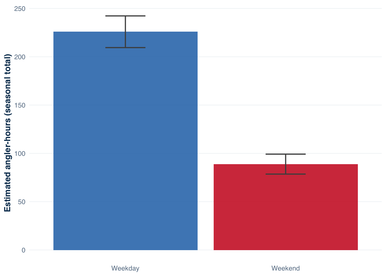
Effort broken down by stratum shows where the season’s angling time was concentrated:
Warning: Count variable angler_count contains 18 zero values.
ℹ Zero values may indicate days with no fishing activity or data collection
  issues.
ℹ Consider whether zeros are true zeros or missing data.
Warning: Count variable expansion_basis contains 21 zero values.
ℹ Zero values may indicate days with no fishing activity or data collection
  issues.
ℹ Consider whether zeros are true zeros or missing data.
Figure 8.1: Seasonal angler-hour estimates with 95% confidence intervals at Harlan Reservoir, by day type. Weekdays accumulate more total effort than weekends because there are roughly 2.5× more eligible weekday days in the season, even though per-day effort is similar across day types. Error bars reflect between-day variability in angler counts scaled by the stratum expansion weight.
Total harvest
estimate_total_harvest() multiplies interview-based harvest rates by the design-weighted effort estimate to produce a season total with variance. It uses the same design object and expansion structure as estimate_effort().
# A tibble: 1 × 5
  estimate    se ci_lower ci_upper     n
     <dbl> <dbl>    <dbl>    <dbl> <int>
1    3259.  365.    2541.    3976.   390
Estimated total harvest across the season is approximately 3,259 fish (95% CI: 2,541–3,976). As with effort, the confidence interval reflects the between-day variability in harvest rates across sampled days.
Catch rate (CPUE)
estimate_catch_rate() returns the ratio-of-means catch per unit effort. Unlike the totals above, CPUE does not use target = "stratum_total" because it is a rate, not a total — it is already expressed per angler-hour and does not need expansion.
Code
cpue <-estimate_catch_rate(harlan_design)
ℹ Using complete trips for CPUE estimation
  (n=390, 65% of 600 interviews) [default]
Code
cpue$estimates
# A tibble: 1 × 5
  estimate     se ci_lower ci_upper     n
     <dbl>  <dbl>    <dbl>    <dbl> <int>
1     1.51 0.0928     1.32     1.69   390
CPUE is 1.51 fish per angler-hour (95% CI: 1.32–1.69). This rate is computed over all species combined and all angler types. Chapter 14 disaggregates CPUE by angler type, by species, and compares the ratio-of-means estimator to the mean-of-ratios alternative.
8.5 A quick results summary
The three estimates can be assembled into a single table. This is the minimum viable results report — a starting point for the fuller reporting format in Chapter 16.
Code
bind_rows( effort$estimates |>select(estimate, se, ci_lower, ci_upper) |>mutate(quantity ="Effort", unit ="angler-hours"), harvest$estimates |>select(estimate, se, ci_lower, ci_upper) |>mutate(quantity ="Total harvest", unit ="fish"), cpue$estimates |>select(estimate, se, ci_lower, ci_upper) |>mutate(quantity ="CPUE", unit ="fish / hr")) |>mutate(estimate =round(estimate, 2),se =round(se, 2),ci_lower =round(ci_lower, 2),ci_upper =round(ci_upper, 2) ) |>select(quantity, unit, estimate, se, ci_lower, ci_upper)
# A tibble: 3 × 6
  quantity      unit         estimate     se ci_lower ci_upper
  <chr>         <chr>           <dbl>  <dbl>    <dbl>    <dbl>
1 Effort        angler-hours  5576.   446.    4694.    6459.
2 Total harvest fish          3259.   365.    2541.    3976.
3 CPUE          fish / hr        1.51   0.09     1.32     1.69
The CV for each estimate — se / estimate × 100 — tells you how precise the estimate is relative to its own scale. An effort CV below 20% is adequate for most management decisions; catch rate CVs are typically higher because they compound uncertainty from both the effort and interview streams.
# A tibble: 3 × 4
  quantity      estimate       se cv_pct
  <chr>            <dbl>    <dbl>  <dbl>
1 Effort         5576.   446.        8
2 Total harvest  3259.   365.       11.2
3 CPUE              1.51   0.0928    6.2
Species composition of harvest
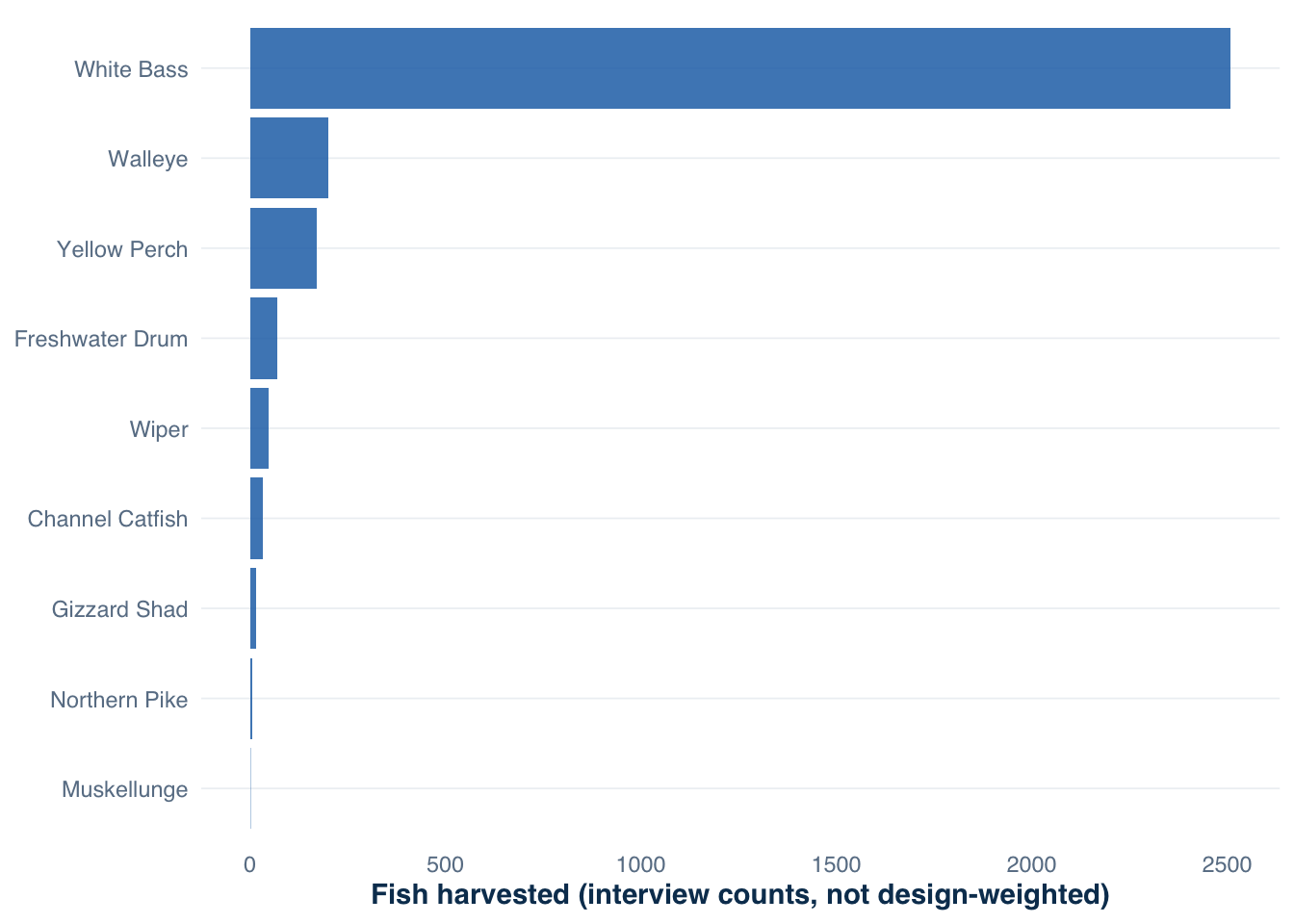
Harvest by species is available directly from the catch table as a raw interview summary. This is not a design-weighted estimate — it represents what the interviewed sample reported, not an expansion to the full season. Chapter 13 produces the design-weighted species-specific harvest totals.
Figure 8.2: Raw interview harvest counts by species at Harlan Reservoir. These are unweighted sums across all interviewed parties — not design-weighted season estimates. The species composition and relative magnitudes are broadly representative of the fishery, but the absolute counts require design-weighting for use in management reporting. See Chapter 13 for weighted species-specific estimates.
Figure 8.2 shows the species composition of angler harvest in the interview sample. White Bass and Walleye dominate. The species mix matters for management: a harvest regulation that targets Walleye — the most regulated species in most Nebraska reservoir fisheries — should be informed by a design-weighted Walleye-specific harvest estimate, not the raw interview count shown here.
Harvest by angler type
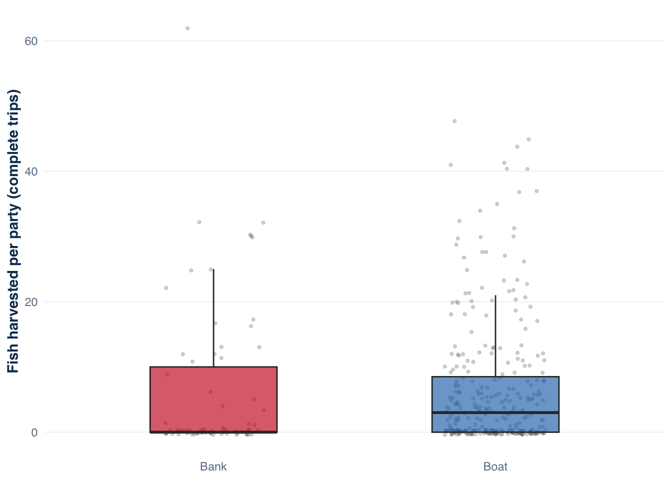
The overall CPUE of 1.51 fish per angler-hour and total harvest of 3,259 fish are fishery-wide averages that pool boat and bank anglers. The interview data show whether those averages conceal important within-fishery differences.
Figure 8.3: Harvest per party by angler type at Harlan Reservoir (completed trips only). Boat anglers tend to harvest more fish per party than bank anglers, with a longer upper tail. Both distributions are strongly right-skewed with many zero-harvest parties. These differences motivate domain-restricted estimates in Chapter 13, which disaggregates the pooled estimates produced in this chapter.
Figure 8.3 shows that boat anglers tend to harvest more fish per party than bank anglers, but both distributions are right-skewed with many zero-harvest parties. Harvest rates that differ between access types mean the pooled estimate in this chapter is a weighted average — weighted by how many angler-hours came from each type. Whether that pooled average is the right quantity for the management question depends on whether the question applies to the whole fishery or to one access type specifically. Chapter 13 demonstrates domain-restricted harvest estimation that produces separate estimates for boat and bank anglers.
8.6 What this chapter skipped
This pipeline produces correct estimates for the Harlan dataset because the dataset was purpose-built to run cleanly. Real data rarely cooperates. The chapters that follow address the complications:
Part II (Survey Designs): how the design choices — access-point vs. roving, shift structure, stratification — affect what the estimates mean and how they are computed.
Chapter 9 (Linked Tables): why the four-table structure is the right format and what goes wrong when tables are collapsed prematurely.
Chapter 10 (Design Object): what the creel_design object stores internally and how to inspect or audit it.
Chapter 11 (Cleaning): how data-quality problems (outlier trips, unrecognized species codes, incomplete trips) affect estimates and how to detect and handle them.
Chapters 12–15 (Estimation): how each estimator works, what assumptions it makes, how to diagnose violations, and how to compute domain-restricted estimates (by species, by angler type, by month).
Chapter 16 (Reporting): how to assemble all estimates into a complete, reproducible report with inline R narrative.
The pipeline here is the skeleton. The rest of the book puts flesh on it.
8.7 Takeaway
Four functions — creel_design(), add_counts(), add_interviews(), add_catch() — build the design object. Three functions — estimate_effort(), estimate_total_harvest(), estimate_catch_rate() — produce the estimates. Everything else in the tidycreel workflow is a variation on this structure: more estimation targets, more diagnostic checks, more domain-restricted summaries.
The numbers from this chapter — 5,576 angler-hours, 3,259 fish harvested, 1.51 fish per angler-hour — are the same numbers that appear throughout Chapters 12–16 as the estimation chapters develop each estimator in detail. Running this pipeline first means the detailed chapters are extending a result you have already seen, not building toward a result you have not.