17  Creel Data as Linked Tables

Keywords

creel survey, fisheries, design-based inference, R, tidycreel, Quarto

17.1 Why creel data resists a single spreadsheet

A creel survey produces at least four distinct kinds of records. The sampling schedule records which days were eligible for sampling and which were actually sampled. Count rounds record how many anglers were observed at each site and time during those sampled days. Interviews record what individual angler parties reported about their trips. Catch records break each party’s report into species-level outcomes.

Each record type answers a different question and belongs to a different observation unit. A count record belongs to a site-period combination. An interview record belongs to an angler party. A catch record belongs to a single species-outcome combination within a single interview. These are different units and should not share rows in the same table.

The practical consequence is statistical. Effort estimators divide an observed angler count by an inclusion probability derived from the schedule. CPUE estimators divide total catch by total angler-hours, where angler-hours come from individual trip records. When the data are stored in a single flat spreadsheet, a join that combines catch with trip records creates duplicate rows — and the denominator for the trip-hours calculation expands with them. The estimate changes not because the underlying data changed but because the data structure changed.

Keeping records in separate tables and joining them only when an analysis requires it is the safest guard against this class of error. This chapter introduces the four Harlan Reservoir survey tables, explains their keys and relationships, and shows how tidycreel validates the structure before any estimation begins.

17.2 The four Harlan tables

The Harlan 2022 creel survey data are distributed across four files, one per record type. Together they cover 211 scheduled days, 236 count observations, 600 angler party interviews, and 987 catch records.

Sampling schedule

The schedule is the sampling frame: the complete list of days that were available to be sampled and a flag for whether each was actually sampled. It is the denominator layer — every inclusion probability calculation for the season traces back to this table.

harlan_schedule

# A tibble: 211 × 4
   date       reservoir        day_type sampled
   <date>     <chr>            <chr>    <lgl>  
 1 2022-04-02 Harlan Reservoir weekend  TRUE   
 2 2022-04-03 Harlan Reservoir weekend  TRUE   
 3 2022-04-04 Harlan Reservoir weekday  FALSE  
 4 2022-04-05 Harlan Reservoir weekday  FALSE  
 5 2022-04-06 Harlan Reservoir weekday  TRUE   
 6 2022-04-07 Harlan Reservoir weekday  TRUE   
 7 2022-04-08 Harlan Reservoir weekday  TRUE   
 8 2022-04-09 Harlan Reservoir weekend  TRUE   
 9 2022-04-10 Harlan Reservoir weekend  FALSE  
10 2022-04-11 Harlan Reservoir weekday  TRUE   
# ℹ 201 more rows

The four columns carry distinct roles. date is the calendar day. reservoir identifies the waterbody — a single schedule can cover multiple reservoirs if they share a survey design. day_type records whether the day was a weekend or weekday, which is the primary stratum in the Harlan design. sampled is the binary flag that separates the realized sample from the non-sampled days in the frame.

harlan_schedule |>
  count(sampled, day_type)

# A tibble: 4 × 3
  sampled day_type     n
  <lgl>   <chr>    <int>
1 FALSE   weekday     68
2 FALSE   weekend     27
3 TRUE    weekday     82
4 TRUE    weekend     34

Of 211 days in the frame, 116 were sampled — roughly 55% of the available days. Weekend and weekday days were sampled at similar rates, reflecting a stratified design where both strata are explicitly covered.

A day that is absent from the schedule cannot be assigned an inclusion probability. Days outside the frame are outside the survey population by definition, so any count or interview record that falls on an unscheduled date is a data quality problem rather than a legitimate observation.

Count records

Count rounds record the instantaneous number of anglers observed at each site during a sampled day. This is the raw observation that gets converted to an estimate of angler effort (Section 20.1). Each row is one count at one site at one moment in time.

harlan_counts

# A tibble: 236 × 9
   reservoir        date       day_type period section count_time   bank_anglers
   <chr>            <date>     <chr>     <dbl> <chr>   <chr>               <int>
 1 Harlan Reservoir 2022-09-02 weekday       1 0       09:00:00:000            0
 2 Harlan Reservoir 2022-09-02 weekday       1 0       11:15:00:000            0
 3 Harlan Reservoir 2022-09-05 weekday       1 0       08:00:00:000            0
 4 Harlan Reservoir 2022-09-05 weekday       1 0       12:15:00:000            0
 5 Harlan Reservoir 2022-09-06 weekday       2 0       13:30:00:000            0
 6 Harlan Reservoir 2022-09-06 weekday       2 0       19:45:00:000            0
 7 Harlan Reservoir 2022-09-08 weekday       1 0       07:00:00:000            0
 8 Harlan Reservoir 2022-09-08 weekday       1 0       13:15:00:000            3
 9 Harlan Reservoir 2022-09-09 weekday       2 0       13:30:00:000            0
10 Harlan Reservoir 2022-09-09 weekday       2 0       18:45:00:000            0
# ℹ 226 more rows
# ℹ 2 more variables: angler_boats <int>, boat_anglers <int>

Four structural columns require explanation. period identifies the count round within the day — in the Harlan design, period 1 is the morning count and period 2 is the afternoon count. section identifies the spatial sub-area of the reservoir that was surveyed; section “0” is a whole-lake count, and other values identify geographic sub-sections. count_time records the exact clock time of the observation, which is used to estimate the fraction of the day each count represents. Together, period, section, and count_time partition the effort counts into the strata and time windows the estimator will sum over.

The three count columns — bank_anglers, angler_boats, and boat_anglers — record observed counts of individual anglers on the bank, boats containing anglers, and the total anglers estimated to be in those boats respectively. boat_anglers is the count used in effort estimation; angler_boats supports boat-party interception rate calculations.

harlan_counts |>
  group_by(period) |>
  summarise(
    n_count_events = n(),
    total_bank     = sum(bank_anglers),
    total_boats    = sum(angler_boats),
    total_boat_ang = sum(boat_anglers),
    .groups = "drop"
  )

# A tibble: 2 × 5
  period n_count_events total_bank total_boats total_boat_ang
   <dbl>          <int>      <int>       <int>          <int>
1      1            120        244        1188           2399
2      2            116        322        1185           2284

The counts table records observed anglers, not interviewed anglers. A high count on a given day does not imply a high number of interviews on that day; a site could be counted without any parties accepting an interview.

Interview records

Each row in the interviews table represents one angler party intercept. The table holds trip-level information: who was sampled, when, how they fished, and how far into their trip they were when the interviewer found them.

harlan_interviews

# A tibble: 600 × 12
   reservoir  date       day_type period section interview_id party_id n_anglers
   <chr>      <date>     <chr>     <dbl> <chr>          <int> <chr>        <dbl>
 1 Harlan Re… 2022-09-01 weekday       2 0                  1 6efcab0…         4
 2 Harlan Re… 2022-09-01 weekday       2 0                  2 d19b214…         3
 3 Harlan Re… 2022-09-01 weekday       2 0                  3 0093195…         3
 4 Harlan Re… 2022-09-01 weekday       2 0                  4 e929b06…         2
 5 Harlan Re… 2022-09-01 weekday       2 0                  5 0c740e9…         2
 6 Harlan Re… 2022-09-01 weekday       2 0                  6 247f59b…         2
 7 Harlan Re… 2022-09-01 weekday       2 0                  7 1ff97fd…         4
 8 Harlan Re… 2022-09-02 weekday       1 0                  8 0bc4a81…         2
 9 Harlan Re… 2022-09-02 weekday       1 0                  9 f0d7c44…         4
10 Harlan Re… 2022-09-02 weekday       1 0                 10 2168ef7…         3
# ℹ 590 more rows
# ℹ 4 more variables: angler_type <chr>, angler_method <chr>,
#   hours_fished <dbl>, trip_status <chr>

Two identifier columns coexist in this table and serve different purposes. party_id is a UUID assigned in the field data system — it is stable across potential data system reloads or imports. interview_id is a sequential integer assigned at analysis time and is the key used to link this table to the catch table. In practice interview_id is simpler to work with; party_id is the audit trail back to the original record in the field system.

trip_status records whether the interview captured a complete trip (the angler had finished fishing) or an incomplete trip (the angler was still fishing when intercepted). This distinction matters for catch estimation: incomplete trip catch cannot simply be summed with complete trip catch without applying a correction for the unobserved portion of the trip.

harlan_interviews |>
  summarise(
    n_interviews     = n(),
    n_sampled_dates  = n_distinct(date),
    complete_trips   = sum(trip_status == "complete"),
    incomplete_trips = sum(trip_status == "incomplete"),
    boat_parties     = sum(angler_type == "boat"),
    bank_parties     = sum(angler_type == "bank"),
    mean_hours       = round(mean(hours_fished), 2)
  )

# A tibble: 1 × 7
  n_interviews n_sampled_dates complete_trips incomplete_trips boat_parties
         <int>           <int>          <int>            <int>        <int>
1          600              91            390              210          322
# ℹ 2 more variables: bank_parties <int>, mean_hours <dbl>

The 600 interviews span 91 sampled dates — not all sampled days yielded interviews, and not all interviews occurred on every sampled day. The mean trip duration across the season was 3.7 hours, though this mixes complete and incomplete trips.

Catch records

The catch table holds one row per species per catch outcome (harvested or released) per interview. There is no trip-level information in this table: interview_id is the only link back to the party, and everything else is species-level.

harlan_catch

# A tibble: 987 × 4
   interview_id species         catch_type n_fish
          <int> <chr>           <chr>       <int>
 1            1 White Bass      released       11
 2            1 White Bass      harvested      32
 3            1 Yellow Perch    released        1
 4            1 Walleye         released        0
 5            4 White Bass      harvested       9
 6            4 Freshwater Drum released        3
 7            5 White Bass      harvested       0
 8            6 Freshwater Drum released        5
 9            8 White Bass      harvested       6
10            8 Freshwater Drum released        1
# ℹ 977 more rows

The structure means a single interview with three species can appear as six rows in the catch table — one harvested and one released row per species. This is intentional. Storing species and outcomes in separate rows keeps the table tidy as species lists expand and makes it straightforward to filter, aggregate, or join by species or outcome.

harlan_catch |>
  group_by(species) |>
  summarise(
    n_records  = n(),
    harvested  = sum(n_fish[catch_type == "harvested"]),
    released   = sum(n_fish[catch_type == "released"]),
    .groups = "drop"
  ) |>
  arrange(desc(harvested + released))

# A tibble: 11 × 4
   species         n_records harvested released
   <chr>               <int>     <int>    <int>
 1 White Bass            376      2509     1919
 2 Walleye               241       200     1699
 3 Freshwater Drum       141        68      702
 4 Yellow Perch           73       169       93
 5 Channel Catfish        60        32      156
 6 Wiper                  49        47       38
 7 Common Carp            19         0       32
 8 Gizzard Shad            5        16        0
 9 Northern Pike          13         6       10
10 Muskellunge             8         1       11
11 Crappie                 2         0        0

Eleven species appear in the catch records for the 2022 Harlan season. White Bass and Walleye dominate the harvest numbers — a pattern consistent with Harlan Reservoir’s well-known walleye fishery and its abundant forage-fish populations.

17.3 Keys and join relationships

The four tables connect through two types of keys. Understanding which key connects which pair of tables is required before any join can be written correctly.

Composite keys link the schedule to the counts and interviews tables. No single column uniquely identifies a sampling event; instead, the combination of reservoir, date, period, and section identifies one count round or one interview occasion. When a count round and an interview occurred at the same site-period, those records carry the same composite key values and can be joined.

Surrogate keys link interviews to catch. The interview_id column is a single integer that uniquely identifies one party intercept and appears in harlan_catch as a foreign key. Every catch row belongs to exactly one interview row.

The join path follows a strict hierarchy:

From	To	Key columns
harlan_schedule	harlan_counts	date, reservoir
harlan_schedule	harlan_interviews	date, reservoir
harlan_counts	harlan_interviews	date, period, section, reservoir
harlan_interviews	harlan_catch	interview_id

The schedule is the root. Counts and interviews are both children of the schedule, connected through shared date and context columns. Catch is a child of interviews, connected through the surrogate key.

Joining in the wrong direction or joining without all required key columns are the two most common sources of phantom rows and silent data loss.

The counts-to-interviews join is worth demonstrating explicitly. It produces one output row per interview, augmented with the count context from the same site-period:

counts_context <- harlan_counts |>
  select(reservoir, date, period, section, bank_anglers, boat_anglers)

interviews_with_context <- left_join(
  harlan_interviews,
  counts_context,
  by = c("reservoir", "date", "period", "section")
)

Warning in left_join(harlan_interviews, counts_context, by = c("reservoir", : Detected an unexpected many-to-many relationship between `x` and `y`.
ℹ Row 1 of `x` matches multiple rows in `y`.
ℹ Row 101 of `y` matches multiple rows in `x`.
ℹ If a many-to-many relationship is expected, set `relationship =
  "many-to-many"` to silence this warning.

# Row count should match interviews exactly
nrow(interviews_with_context) == nrow(harlan_interviews)

[1] FALSE

interviews_with_context |>
  select(interview_id, date, period, section, hours_fished, bank_anglers, boat_anglers) |>
  head(5)

# A tibble: 5 × 7
  interview_id date       period section hours_fished bank_anglers boat_anglers
         <int> <date>      <dbl> <chr>          <dbl>        <int>        <int>
1            1 2022-09-01      2 0               5.36            5           33
2            1 2022-09-01      2 0               5.36            2           11
3            2 2022-09-01      2 0               1.1             5           33
4            2 2022-09-01      2 0               1.1             2           11
5            3 2022-09-01      2 0               8.31            5           33

The row count is preserved — one output row per interview — and each interview row now carries the angler count from the concurrent count round. A mismatch in row count would indicate either an interview with no corresponding count or multiple count rounds matching the same interview key.

17.4 Validating joins

Because the tables are linked by keys, each join can be tested before it is used in estimation. The standard tests are anti-joins (finding unmatched records on either side) and row-count comparisons (confirming that joins expand or contract the row count as expected).

Catch records without interviews

Every catch row should trace back to a real interview. An orphan catch record — one whose interview_id does not exist in the interviews table — indicates either a data entry error or a deleted interview that left catch records behind.

orphan_catch <- anti_join(harlan_catch, harlan_interviews, by = "interview_id")
nrow(orphan_catch)

[1] 0

Zero orphans. Every catch record in the 2022 Harlan data has a matching interview. This check is not guaranteed to pass on data from other projects or other years, so it should be part of any standard data preparation script.

Interviews without catch records

The reverse anti-join finds interviews that produced no catch records. This is expected — anglers who caught nothing or refused to report catch produce an interview row but no corresponding catch rows. The number should be interpretable given the fishery.

no_catch_interviews <- anti_join(
  harlan_interviews,
  harlan_catch,
  by = "interview_id"
)

no_catch_interviews |>
  count(trip_status, name = "n_interviews")

# A tibble: 2 × 2
  trip_status n_interviews
  <chr>              <int>
1 complete              56
2 incomplete           102

Of the 600 interviews, 158 produced no catch records. The breakdown by trip_status shows that most of these are incomplete trips. Parties still fishing when intercepted often had not yet landed fish, so the absence of catch records is consistent with the data — not an error. Section 19.7 covers how to handle incomplete-trip catch in the estimation step.

Schedule versus counts

Count records should come from days that the schedule marks as sampled. A count date that is absent from the schedule as a sampled day suggests either a data entry error in the schedule or an unsanctioned extra sampling day.

sampled_dates <- harlan_schedule |>
  filter(sampled) |>
  pull(date)

harlan_counts |>
  filter(!date %in% sampled_dates) |>
  distinct(date, reservoir)

# A tibble: 2 × 2
  date       reservoir       
  <date>     <chr>           
1 2022-10-30 Harlan Reservoir
2 2022-04-01 Harlan Reservoir

Two count dates fall outside the set of days marked as sampled in the Harlan schedule. In a flat file these two dates would be indistinguishable from the rest of the count records. In the linked-table structure, the discrepancy surfaces in two lines of code. Whether the correct response is to add those dates to the schedule or to remove the counts is a domain decision; the structure makes the problem findable.

17.5 Validating tables with validate_creel_data()

tidycreel provides validate_creel_data() to run a systematic battery of checks on count and interview tables. It verifies column types, flags impossible values (negative counts, implausible dates, NA values in identifier fields), and reports the result as a structured pass/warn/fail summary.

validate_creel_data(
  counts     = harlan_counts,
  interviews = harlan_interviews
)

── Creel Data Validation ───────────────────────────────────────────────────────

63 pass | 0 warn | 0 fail

── Table: counts ──

✔ reservoir

✔ type: class: character

✔ na_rate: 0 / 236 NA (0%)

✔ empty_strings: none

✔ date

✔ type: class: Date

✔ na_rate: 0 / 236 NA (0%)

✔ date_range: all within 1970-01-01 - 2100-12-31

✔ day_type

✔ type: class: character

✔ na_rate: 0 / 236 NA (0%)

✔ empty_strings: none

✔ period

✔ type: class: numeric

✔ na_rate: 0 / 236 NA (0%)

✔ negative_values: none

✔ section

✔ type: class: character

✔ na_rate: 0 / 236 NA (0%)

✔ empty_strings: none

✔ count_time

✔ type: class: character

✔ na_rate: 0 / 236 NA (0%)

✔ empty_strings: none

✔ bank_anglers

✔ type: class: integer

✔ na_rate: 0 / 236 NA (0%)

✔ negative_values: none

✔ angler_boats

✔ type: class: integer

✔ na_rate: 0 / 236 NA (0%)

✔ negative_values: none

✔ boat_anglers

✔ type: class: integer

✔ na_rate: 0 / 236 NA (0%)

✔ negative_values: none

── Table: interviews ──

✔ reservoir

✔ type: class: character

✔ na_rate: 0 / 600 NA (0%)

✔ empty_strings: none

✔ date

✔ type: class: Date

✔ na_rate: 0 / 600 NA (0%)

✔ date_range: all within 1970-01-01 - 2100-12-31

✔ day_type

✔ type: class: character

✔ na_rate: 0 / 600 NA (0%)

✔ empty_strings: none

✔ period

✔ type: class: numeric

✔ na_rate: 0 / 600 NA (0%)

✔ negative_values: none

✔ section

✔ type: class: character

✔ na_rate: 0 / 600 NA (0%)

✔ empty_strings: none

✔ interview_id

✔ type: class: integer

✔ na_rate: 0 / 600 NA (0%)

✔ negative_values: none

✔ party_id

✔ type: class: character

✔ na_rate: 0 / 600 NA (0%)

✔ empty_strings: none

✔ n_anglers

✔ type: class: numeric

✔ na_rate: 0 / 600 NA (0%)

✔ negative_values: none

✔ angler_type

✔ type: class: character

✔ na_rate: 0 / 600 NA (0%)

✔ empty_strings: none

✔ angler_method

✔ type: class: character

✔ na_rate: 0 / 600 NA (0%)

✔ empty_strings: none

✔ hours_fished

✔ type: class: numeric

✔ na_rate: 0 / 600 NA (0%)

✔ negative_values: none

✔ trip_status

✔ type: class: character

✔ na_rate: 0 / 600 NA (0%)

✔ empty_strings: none

The Harlan data passes all 63 checks with no warnings and no failures. This outcome is worth recording at the start of any analysis session: a passing run confirms the tables have not been modified in a way that would silently break downstream estimation. A failure identifies specific columns and rows to investigate before estimation proceeds.

The checks validate_creel_data() runs are not redundant with the anti-joins in Section 17.4. The anti-joins test relational integrity between tables. The validation function tests internal integrity within each table: whether a date column contains actual dates, whether angler counts contain negative numbers, whether identifier columns have unexpected missing values. Both sets of checks should pass before estimation begins.

17.6 Formalizing the schema with creel_schema()

creel_schema() records the mapping from your column names to the conceptual roles that tidycreel estimation functions expect. Survey data rarely arrives with column names that match package conventions. Rather than forcing users to rename columns in every function call, the schema holds the mapping once and passes it forward.

harlan_schema <- creel_schema(
  survey_type        = "instantaneous",
  interviews_table   = "harlan_interviews",
  counts_table       = "harlan_counts",
  catch_table        = "harlan_catch",
  date_col           = "date",
  effort_col         = "hours_fished",
  trip_status_col    = "trip_status",
  interview_uid_col  = "interview_id",
  bank_anglers_col   = "bank_anglers",
  angler_boats_col   = "angler_boats",
  n_anglers_col      = "n_anglers",
  angler_type_col    = "angler_type",
  angler_method_col  = "angler_method",
  species_col        = "species",
  catch_count_col    = "n_fish",
  catch_type_col     = "catch_type"
)

harlan_schema

<creel_schema: instantaneous>

── interviews: harlan_interviews ──

date -> date
effort -> hours_fished
trip_status -> trip_status
n_anglers -> n_anglers
angler_type -> angler_type
angler_method -> angler_method
interview_uid -> interview_id

── counts: harlan_counts ──

bank_anglers -> bank_anglers
angler_boats -> angler_boats

── catch: harlan_catch ──

species -> species
catch_count -> n_fish
catch_type -> catch_type

The printed schema shows which column in each table maps to which conceptual role. effort -> hours_fished means that the hours_fished column in the interviews table carries the trip-duration information the estimator uses. catch_count -> n_fish means that n_fish in the catch table is the count column.

Schemas are useful because the data are in separate tables. If all columns were in one flat file, distinguishing between hours_fished (trip-level) and n_fish (catch-level) would require column-name conventions rather than table structure.

In the next chapter, the schema is consumed by creel_design() to produce the design object that estimation functions take as their primary argument.

17.7 Standardizing columns with prep_interview_catch()

tidycreel includes a family of prep_* functions that standardize column names within individual tables before passing them to the package internals. prep_interview_catch() handles the catch table.

prepped_catch <- prep_interview_catch(
  data          = harlan_catch,
  interview_uid = "interview_id",
  species       = "species",
  count         = "n_fish",
  catch_type    = "catch_type"
)

prepped_catch

# A tibble: 987 × 4
   interview_uid species         count catch_type
           <int> <chr>           <int> <chr>     
 1             1 White Bass         11 released  
 2             1 White Bass         32 harvested 
 3             1 Yellow Perch        1 released  
 4             1 Walleye             0 released  
 5             4 White Bass          9 harvested 
 6             4 Freshwater Drum     3 released  
 7             5 White Bass          0 harvested 
 8             6 Freshwater Drum     5 released  
 9             8 White Bass          6 harvested 
10             8 Freshwater Drum     1 released  
# ℹ 977 more rows

The output carries standardized names — interview_uid, species, count, catch_type — that the internal estimation pipeline expects. Running prep_interview_catch() at the start of an analysis session means that column name differences between projects do not propagate into estimation errors.

The prep functions are thin wrappers: they rename columns and return the data with the same number of rows. They do not validate values, impute missing data, or recode factors. Validation (via validate_creel_data()) and join checking (via anti-joins) should run before the prep step, not after it.

17.8 The danger of premature flattening

The most common data management mistake in creel analysis is joining tables before the analysis requires it. The typical failure mode is joining interviews to catch before aggregating catch to the party level. The interview table has one row per party. The catch table has one row per species per outcome per party. The join expands the interview table, and any trip-level statistic computed on the result uses the wrong denominator.

interviews_flat <- left_join(
  harlan_interviews,
  harlan_catch,
  by = "interview_id"
)

tibble(
  source   = c("harlan_interviews", "harlan_catch", "flat join"),
  n_rows   = c(nrow(harlan_interviews), nrow(harlan_catch), nrow(interviews_flat))
)

# A tibble: 3 × 2
  source            n_rows
  <chr>              <int>
1 harlan_interviews    600
2 harlan_catch         987
3 flat join           1145

The flat join produces 1145 rows from an interview table with 600 rows. Interviews with multiple species-outcome combinations appear multiple times. To see how many times each interview appears:

interviews_flat |>
  count(interview_id, name = "n_rows_in_join") |>
  count(n_rows_in_join, name = "n_interviews")

# A tibble: 6 × 2
  n_rows_in_join n_interviews
           <int>        <int>
1              1          308
2              2          139
3              3           81
4              4           48
5              5           20
6              6            4

Most interviews appear more than once in the flat join. An interview that reported three species with two outcomes each would appear six times. If trip-level effort hours are then averaged on the flat file, the denominator is inflated and the mean is wrong:

tibble(
  calculation = c("interview table (correct)", "flat join (wrong)"),
  mean_hours  = c(
    mean(harlan_interviews$hours_fished),
    mean(interviews_flat$hours_fished)
  )
)

# A tibble: 2 × 2
  calculation               mean_hours
  <chr>                          <dbl>
1 interview table (correct)       3.68
2 flat join (wrong)               4.44

The correct pattern is to aggregate catch to the party level first, then join. The resulting joined table has the same row count as the interview table.

catch_by_interview <- harlan_catch |>
  group_by(interview_id) |>
  summarise(
    total_fish     = sum(n_fish),
    species_caught = n_distinct(species[n_fish > 0]),
    .groups = "drop"
  )

interviews_with_catch <- left_join(
  harlan_interviews,
  catch_by_interview,
  by = "interview_id"
)

nrow(interviews_with_catch)

[1] 600

Aggregating before joining preserves the one-row-per-party structure:

interviews_with_catch |>
  select(interview_id, date, angler_type, hours_fished, total_fish, species_caught) |>
  head(5)

# A tibble: 5 × 6
  interview_id date       angler_type hours_fished total_fish species_caught
         <int> <date>     <chr>              <dbl>      <int>          <int>
1            1 2022-09-01 boat                5.36         44              2
2            2 2022-09-01 bank                1.1          NA             NA
3            3 2022-09-01 bank                8.31         NA             NA
4            4 2022-09-01 boat                5.96         12              2
5            5 2022-09-01 boat                4.33          0              0

The row count matches the interview table and each row carries trip-level effort alongside party-level catch totals. This is the correct shape for CPUE calculation: one row per trip, with hours and catch from the same observation unit.

17.9 Visualizing the data hierarchy

Record counts across tables

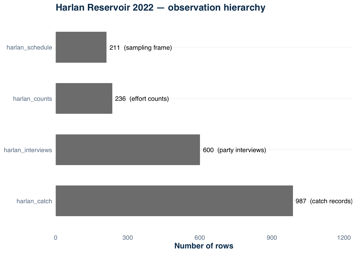
The observation hierarchy is clearest when the row counts are shown together. Each table is a different resolution of the same survey: one sampled day produces multiple count events, those count events coincide with multiple interviews, and each interview yields multiple catch records.

record_counts <- tibble(
  table = c("harlan_schedule", "harlan_counts", "harlan_interviews", "harlan_catch"),
  n     = c(nrow(harlan_schedule), nrow(harlan_counts), nrow(harlan_interviews), nrow(harlan_catch)),
  role  = c("sampling frame", "effort counts", "party interviews", "catch records")
) |>
  mutate(table = fct_inorder(table))

ggplot(record_counts, aes(x = n, y = fct_rev(table), fill = role)) +
  geom_col(width = 0.6) +
  geom_text(
    aes(label = paste0(n, "  (", role, ")")),
    hjust = -0.05, size = 3.2
  ) +
  scale_fill_manual(values = creel_palette(4), guide = "none") +
  scale_x_continuous(expand = expansion(mult = c(0, 0.25))) +
  labs(
    x     = "Number of rows",
    y     = NULL,
    title = "Harlan Reservoir 2022 — observation hierarchy"
  ) +
  theme_creel()

Warning: No shared levels found between `names(values)` of the manual scale and the
data's fill values.
No shared levels found between `names(values)` of the manual scale and the
data's fill values.

Figure 17.1: Row counts for the four Harlan survey tables. Each table represents a different observation unit. The increasing counts from schedule to catch reflect the one-to-many relationships in the join hierarchy.

The schedule and counts rows are similar in number — 211 and 236 respectively — because a typical sampled day produces only a few count events (one per period per section). Interviews are more numerous at 600 because multiple parties are intercepted per count round. Catch records are the most numerous at 987 because each interview can produce records for multiple species and outcomes.

Coverage: which sampled days appear in each table?

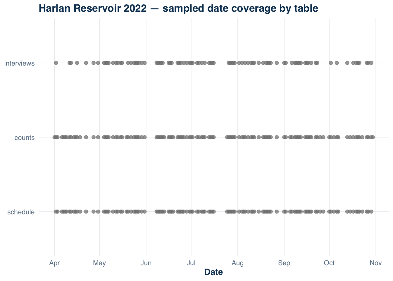
Not every sampled day produces both counts and interviews. Plotting date coverage reveals where data are dense and where they are sparse — and makes it immediately visible that the three tables do not share identical date ranges.

coverage_data <- bind_rows(
  harlan_schedule |>
    filter(sampled) |>
    transmute(date, source = "schedule"),
  harlan_counts |>
    distinct(date) |>
    mutate(source = "counts"),
  harlan_interviews |>
    distinct(date) |>
    mutate(source = "interviews")
) |>
  mutate(source = factor(source, levels = c("schedule", "counts", "interviews")))

ggplot(coverage_data, aes(x = date, y = source, color = source)) +
  geom_point(size = 1.8, alpha = 0.7) +
  scale_color_manual(values = creel_palette(3), guide = "none") +
  scale_x_date(date_breaks = "1 month", date_labels = "%b") +
  labs(
    x     = "Date",
    y     = NULL,
    title = "Harlan Reservoir 2022 — sampled date coverage by table"
  ) +
  theme_creel() +
  theme(panel.grid.major.x = element_line(linewidth = 0.3))

Warning: No shared levels found between `names(values)` of the manual scale and the
data's colour values.

Figure 17.2: Date coverage across the schedule (sampled days), counts, and interview tables for Harlan Reservoir 2022. Points indicate days with records in each table. Days that appear in the schedule but not in counts or interviews indicate sampled days with no recorded activity.

Several dates appear in the schedule and counts rows but not in the interviews row. A day can be counted without any parties agreeing to be interviewed. The figure makes this gap visible. Treating the interview date range as equivalent to the sampled date range would overstate the survey frame and understate the non-response rate.

17.10 Table ownership rules

A relational model fails when the same information lives in multiple tables and the copies diverge. Each table should own its fields exclusively — any column that appears in two tables is a candidate for inconsistency over time.

The ownership assignments for a creel survey are driven by observation unit:

Schedule owns date-level information: which dates were in the frame, their day_type, and whether they were sampled. No other table should store day_type as an original column; if counts or interviews need day_type, they should derive it by joining to the schedule rather than by maintaining their own copy. In the Harlan data, day_type appears in both harlan_counts and harlan_interviews as a convenience column. Verifying that these copies are consistent with the schedule is a mandatory check:

# Check that day_type in counts matches schedule
left_join(
  harlan_counts |> select(date, day_type_counts = day_type),
  harlan_schedule |> select(date, day_type_schedule = day_type),
  by = "date"
) |>
  filter(day_type_counts != day_type_schedule) |>
  nrow()

[1] 0

Zero mismatches — the day_type copies in Harlan counts are consistent with the schedule. This check costs one join and should be part of any data preparation script. If mismatches exist, the schedule is the authoritative source and the copies in counts and interviews should be corrected by joining from the schedule, not by hand-editing individual rows.

Counts own site-period-level observations: the number of anglers of each type seen at a given section during a given count round. They do not own interview counts or any trip-level information.

Interviews own party-level trip information: interception time, trip duration, method, angler type, and trip completion status. They do not own species-level catch. If an interview table contains a column for total catch by species, that total will diverge from the sum of the catch table whenever catch records are edited after the fact.

Catch owns species-level outcomes for each interview. It holds interview_id as a foreign key but not any other trip-level columns. If catch records carry hours_fished or date copied from the interview, edits to the interview no longer propagate to the catch copies, and a join will produce two different values for the same attribute.

Violations of these rules are common in creel programs that began as spreadsheets and were later imported into a data system. Columns get copied as a convenience and then diverge. The linked-table approach makes these copies unnecessary: the information is always available through a join from the table that owns it.

17.11 Common mistakes

Two mistakes recur in creel data management that are not fully covered by the examples above.

Silent loss from inner joins. An inner join between interviews and catch drops the 158 Harlan interviews that have no catch records. Those parties fished — their effort hours belong in the CPUE denominator. Dropping them biases CPUE upward. The correct join is always a left join from interviews to catch; the NA values that appear for no-catch parties are informative and should be replaced with zero fish, not removed.

Confusion between counts and interview denominators. After the counts-to- interviews join demonstrated in Section 17.3, the joined table carries both bank_anglers (from counts — all anglers visible at the site) and n_anglers (from interviews — anglers in the intercepted party). These are different quantities. bank_anglers is the instantaneous census; n_anglers is the party size. Using the wrong column in an effort estimator produces a result that appears numerically plausible but is conceptually wrong. Keeping the columns in separate tables before joining makes the distinction visible; a flat file obscures it.

17.12 Takeaway

Creel data is naturally relational. The sampling frame, effort counts, party interviews, and species-level catch records each describe a different observation unit and belong in separate tables with stable keys connecting them.

Keeping these tables separate until the analysis requires them protects the row counts and denominators that estimators depend on. It also makes data quality problems discoverable: orphan catch records, count dates outside the schedule frame, and interview dates that do not match sampled days all surface through explicit join checks rather than manifesting silently as wrong estimates.

tidycreel supports this structure through validate_creel_data(), which checks internal integrity within each table, and creel_schema(), which formalizes the column mapping that estimation functions consume. The next chapter uses both to construct the creel_design object.