creel survey, fisheries, design-based inference, R, tidycreel, Quarto
22.1 Three quantities, one fishery
Effort is the foundation of creel estimation, but managers usually ask about catch, harvest, and species. Those questions sound similar but they require different estimators and different data columns.
Catch is the total number of fish that left the water during a fishing trip, regardless of what happened to them afterward. A walleye that was measured and returned is a caught fish. So is one that went in the livewell. Catch includes both harvest and release.
Harvest is the subset of catch that anglers retained — fish taken home, eaten, or otherwise removed from the fishery permanently. Harvest is the quantity most directly tied to fishing mortality, and it is what regulations target when they set bag limits or size restrictions.
Release is the complement: fish caught and returned. Release is more subject to measurement error than harvest because creel clerks can inspect retained fish directly but must rely on angler recall for fish already back in the water. Access-point surveys reduce this error by interviewing anglers immediately after they leave the water, when memory of released fish is still fresh (Pollock et al. 1994).
The distinction matters. An angler who catches fifteen white bass but keeps only three contributes a harvest total of three and a release total of twelve, even though the trip produced one catch total of fifteen. The estimator and its denominator have to match the question being answered.
This chapter shows how the Harlan Reservoir 2022 survey data produce estimates of all three quantities using tidycreel, and how the relationship between them reveals the character of the fishery.
22.2 The harvest estimator
Total harvest is estimated as the product of total angling effort and a per-unit-effort rate. The rate is the harvest per unit effort (HPUE):
where \widehat{E}_j is the estimated total angling effort in stratum j (angler-hours) and \widehat{\text{HPUE}}_j is the ratio-of-means HPUE for that stratum. The season total sums across strata:
\widehat{H} = \sum_j \widehat{H}_j
with variance propagated through the delta method, combining uncertainty from both the effort and HPUE estimates.
The ratio-of-means HPUE is defined as total observed harvest divided by total observed effort across all interviews in a stratum (Pollock et al. 1994; Hoenig et al. 1997):
where h_i is fish harvested on trip i and l_i is hours fished. estimate_harvest_rate() defaults to completed trips, matching the CPUE estimator. Harvest from an incomplete trip is theoretically observable — what is in the livewell at interview time is harvested regardless of whether the angler keeps fishing — but using the same interview pool as CPUE makes the HPUE + RPUE ≈ CPUE consistency check exact rather than approximate.
The same product structure applies to release: \widehat{R}_j = \widehat{E}_j \times \widehat{\text{RPUE}}_j, and to total catch: \widehat{C}_j = \widehat{E}_j \times \widehat{\text{CPUE}}_j. Because all three rate estimators default to the same completed-trip interview pool, the season totals satisfy \widehat{C} \approx \widehat{H} + \widehat{R} up to rounding. Roving designs use a mean-of-ratios estimator; see Chapter 17 for that case.
22.3 Preparing catch data for estimation
The design construction in this chapter differs from Section 21.6 in one important respect. That section passed a single harvest column to add_interviews() as the catch argument. Here, we need separate quantities for total catch and harvest. Released fish follow automatically from their difference.
The harlan_catch table stores species-level fish counts with a catch_type column that takes values "harvested" or "released". Pivot that table to one row per interview with separate columns for each type.
The result has one row per interview that recorded at least one fish. When we join it to the full interview table, any missing interview receives zeros for all three columns.
The interview table now carries three catch columns at the trip level. Each feeds a different estimation function downstream.
22.4 Building the design object
With three catch columns available, the design pipeline is identical to Section 21.6 except that we now pass both catch and harvest to add_interviews(). The harvest argument tells tidycreel which column represents retained fish.
Count data preparation mirrors Section 21.6: shift lengths convert instantaneous angler counts to angler-hours, so effort and rates share the same time units.
22.5 Harvest rates by day type
The harvest rate — fish harvested per angler-hour — is the ratio-of-means HPUE from 390 completed-trip interviews. estimate_harvest_rate() defaults to completed trips, matching the CPUE estimator (see Section 22.2).
Code
estimate_harvest_rate(harlan_design_ch13)
ℹ Filtering to complete trips for HPUE estimation
  (n=390, 65% of 600 interviews) [default]
── Creel Survey Estimates ──────────────────────────────────────────────────────
Method: Ratio-of-Means HPUE
Variance: Taylor linearization
Confidence level: 95%
Unit: fish/angler-hour

# A tibble: 1 × 5
  estimate     se ci_lower ci_upper     n
     <dbl>  <dbl>    <dbl>    <dbl> <int>
1    0.585 0.0464    0.495    0.676   390
The overall Harlan 2022 harvest rate is 0.585 fish per angler-hour (95% CI: 0.495–0.676). Disaggregating by day type shows that weekend anglers harvest at a substantially higher rate than weekday anglers:
Code
estimate_harvest_rate(harlan_design_ch13, by = day_type)
ℹ Filtering to complete trips for HPUE estimation
  (n=390, 65% of 600 interviews) [default]
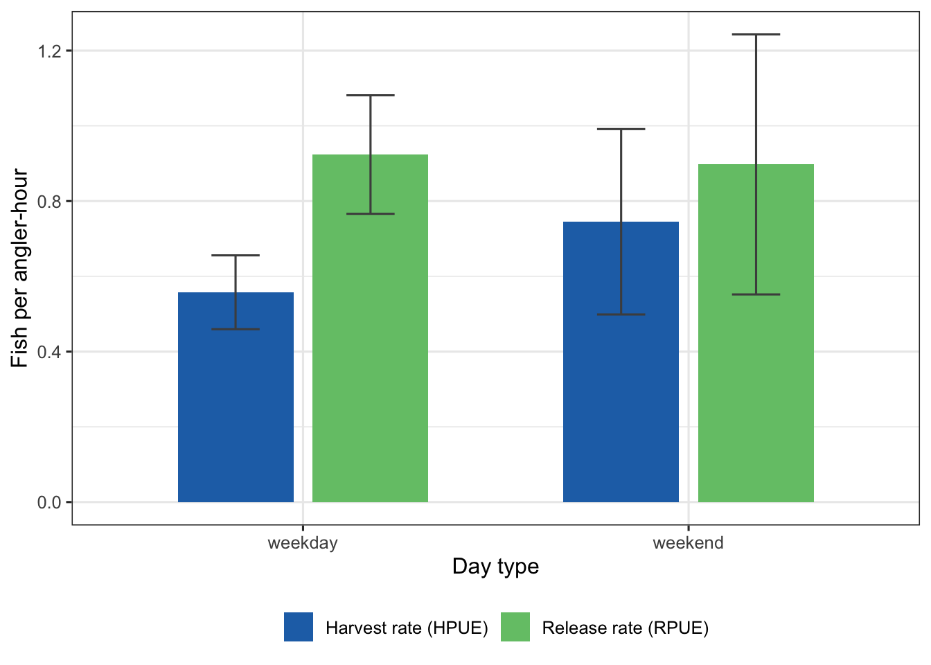
Figure 22.1: Estimated harvest rate (HPUE) and release rate (RPUE) by day type at Harlan Reservoir, 2022. Bars show the ratio-of-means estimate from completed-trip interviews; error bars show 95% confidence intervals. Weekend anglers harvested at a noticeably higher rate than weekday anglers, while release rates were similar across day types.
The weekend harvest rate (0.745 fish/hour, 95% CI: 0.499–0.991) is about 33% higher than weekdays (0.558, 95% CI: 0.459–0.656). Release rates are nearly identical — 0.924 on weekdays and 0.897 on weekends. Weekend anglers both catch more (CPUE: 1.64 vs 1.48 fish/hr weekday) and retain a larger fraction of what they catch. The weekend fishery at Harlan draws more anglers actively targeting harvestable species, while weekday fishing is often more incidental in character.
The stratum-specific rates matter because they multiply against different effort volumes to produce the season harvest totals. A higher per-hour rate on weekends does not mean weekends dominate the harvest — that depends on how many angler-hours each stratum contributes.
22.6 Estimating total harvest
estimate_total_harvest() combines effort and HPUE via the delta method. The target argument controls which effort domain is multiplied by the rate: "sampled_days" (days when at least one count occurred) or "stratum_total" (all days in the stratum, sampled or not). Use "stratum_total" when reporting seasonal harvest for the full fishery.
Code
estimate_total_harvest(harlan_design_ch13)
── Creel Survey Estimates ──────────────────────────────────────────────────────
Method: Total Harvest (Effort × HPUE)
Variance: Taylor linearization
Confidence level: 95%
Effort target: sampled_days
Unit: fish
Party-size expansion SE: 286.8 (included in se)
# A tibble: 1 × 5
estimate se ci_lower ci_upper n
<dbl> <dbl> <dbl> <dbl> <int>
1 12692. 1780. 9193. 16191. 390
── Creel Survey Estimates ──────────────────────────────────────────────────────
Method: Total Harvest (Effort × HPUE)
Variance: Taylor linearization
Confidence level: 95%
Effort target: stratum_total
Unit: fish
Party-size expansion SE: 514.9 (included in se)
# A tibble: 1 × 5
estimate se ci_lower ci_upper n
<dbl> <dbl> <dbl> <dbl> <int>
1 22783. 2577. 17715. 27850. 390
On sampled days only, estimated harvest was 11,052 fish (95% CI: 8,092–14,012). Expanding to all days in the season yields 19,825 fish (95% CI: 14,649–25,000). The difference reflects the unsampled days: the creel did not cover every day on the calendar, but the expansion assumes those days had fishing activity at the same rate structure as sampled days. The sampled-days total describes what happened on surveyed days; the stratum-total estimates season-level removal from the stock.
Grouping by day type connects the rates from Section 22.5 to the season totals:
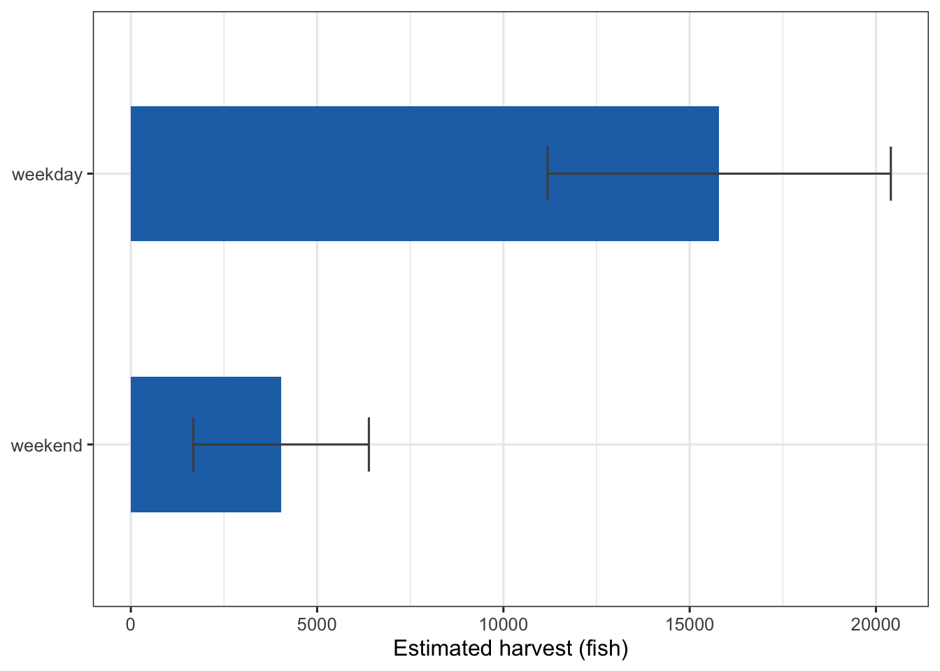
Figure 22.2: Estimated season harvest by day type at Harlan Reservoir, 2022, using the stratum-total effort expansion. Error bars show 95% confidence intervals. Despite weekends having a higher harvest rate per angler-hour, weekdays contribute roughly four times more harvest in absolute terms because weekday fishing pressure is substantially greater.
Weekdays account for roughly four times more harvest than weekends in absolute terms (15,793 vs. 4,032 fish). Even though the per-hour harvest rate is higher on weekends, weekday effort at Harlan is substantially larger — enough to reverse the relationship between rate and total. This is the harvest analog of the effort result from Section 21.9: a higher rate does not guarantee a higher total when the two strata differ in total effort by a wide margin.
22.7 Estimating total catch and release
Harvest and release are the two components of total catch. Estimating each separately allows the analyst to report how much fishing activity ended with fish returned to the water — an increasingly important management metric in fisheries where exploitation targets are low or catch-and-release is promoted.
── Creel Survey Estimates ──────────────────────────────────────────────────────
Method: product-total-release
Variance: Taylor linearization
Confidence level: 95%
Effort target: stratum_total
Unit: fish
Party-size expansion SE: 810.1 (included in se)
# A tibble: 1 × 5
estimate se ci_lower ci_upper n
<dbl> <dbl> <dbl> <dbl> <int>
1 35845. 4082. 27819. 43872. 390
The estimated total catch for the 2022 season was 49,756 fish (95% CI: 37,272–62,239). Of that, approximately 19,825 were harvested and 30,310 released — roughly 60% of all fish caught were returned. That is a large catch-and-release fraction, and it raises a question the estimate alone cannot answer: do those released fish survive? The creel measures the number returned; post-release mortality is a separate quantity requiring tagging studies or laboratory experiments and is applied outside the creel workflow.
The catch rate (CPUE) and release rate (RPUE) confirm the partition:
Code
estimate_release_rate(harlan_design_ch13)
ℹ Filtering to complete trips for RPUE estimation
  (n=390, 65% of 600 interviews) [default]
── Creel Survey Estimates ──────────────────────────────────────────────────────
Method: ratio-of-means-rpue
Variance: Taylor linearization
Confidence level: 95%
Unit: fish/angler-hour

# A tibble: 1 × 5
  estimate     se ci_lower ci_upper     n
     <dbl>  <dbl>    <dbl>    <dbl> <int>
1    0.920 0.0733    0.776     1.06   390
Code
estimate_catch_rate(harlan_design_ch13)
ℹ Using complete trips for CPUE estimation
  (n=390, 65% of 600 interviews) [default]
── Creel Survey Estimates ──────────────────────────────────────────────────────
Method: Ratio-of-Means CPUE
Variance: Taylor linearization
Confidence level: 95%
Unit: fish/angler-hour

# A tibble: 1 × 5
  estimate     se ci_lower ci_upper     n
     <dbl>  <dbl>    <dbl>    <dbl> <int>
1     1.51 0.0928     1.32     1.69   390
All three rate estimators (estimate_catch_rate(), estimate_harvest_rate(), estimate_release_rate()) default to the 390 completed-trip interviews (65% of 600 parties). Using the same interview pool makes the consistency check exact: HPUE (0.585) + RPUE (0.920) = 1.505, which rounds to CPUE (1.51), confirming the catch partition is internally coherent.
22.8 Reporting catch, harvest, and release together
Management reports often need all three quantities in a single table with consistent confidence intervals. Collect the stratum-total estimates for each and bind them by row.
# A tibble: 3 × 6
  quantity      estimate    se ci_lower ci_upper     n
  <chr>            <dbl> <dbl>    <dbl>    <dbl> <int>
1 Total harvest    22783  2577    17715    27850   390
2 Total release    35845  4082    27819    43872   390
3 Total catch      58628  5977    46878    70378   390
The combined table expresses the accounting identity of the fishery: catch equals harvest plus release. The estimates do not sum exactly because the component estimators differ slightly in their interview pools and variance calculations, but they share the same effort base and the same interview records.
When presenting this table in a management report, the relevant context is what the estimates imply for fishing mortality. An estimated 19,825 harvested fish represents direct removal from the Harlan population in 2022 — the number an exploitation rate or yield model requires as input. The 30,310 released fish contribute to fishing mortality only through post-release mortality, a species-specific quantity not estimated by the creel.
22.9 Species composition of the harvest
The estimates above report totals across all species combined. Species-specific harvest estimates require species-level catch rates from estimate_catch_rate(by = species), which Section 23.2 covers in detail. For composition analysis — understanding which species anglers encounter and what fraction they retain — the raw catch table is the right tool. It records the actual species and catch type for every fish without expansion to the population level.
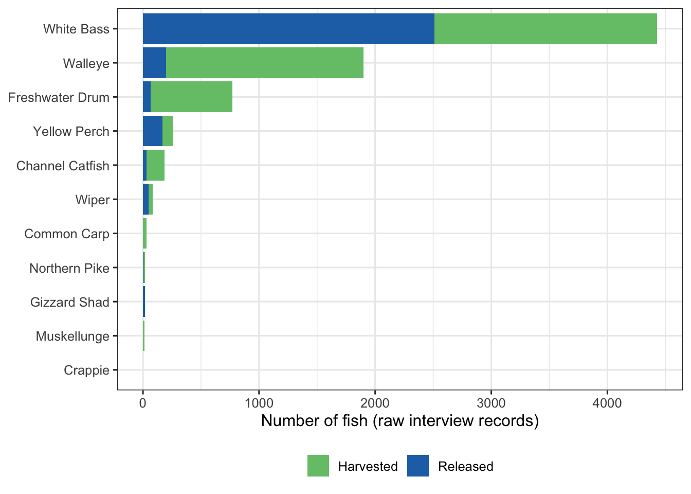
White bass dominate by both total catch (4,428 fish) and harvest (2,509), with 43% released. Walleye show a starkly different pattern: 1,899 fish caught, 200 retained, 89.5% released. Freshwater drum are similarly high at 91% released. These patterns reflect angler preference and regulation structure: walleye have a size limit and are a prized food fish, so sub-legal fish are released; freshwater drum are often returned regardless of size. Gizzard shad show 0% released — every shad caught was harvested, consistent with their use as cut bait.
Figure 22.3: Species catch composition at Harlan Reservoir, 2022. Bars show recorded fish counts from interview catch records, split by harvest (blue) and release (green). Species are ordered by total catch. White bass dominate both harvest and total catch; walleye and freshwater drum show high release fractions consistent with size-limit regulations and angler preferences.
The species composition in raw catch records describes which species anglers encounter and what they do with them. It does not, by itself, produce an expanded season total per species — that requires design-based species-level CPUE estimates applied to total effort, which Section 23.2 covers using estimate_catch_rate(by = species).
22.10 What the creel can and cannot measure
A well-executed creel survey provides design-unbiased estimates of harvest, catch, and release at the stratum level. Three limitations are worth stating clearly.
Post-release mortality is not measured. The creel records that a fish was returned to the water; it does not follow that fish. For species with high post-release survival under typical conditions (most warm-water species in summer), the released total approximates the number that survive. For species with elevated post-release mortality — fish caught on bait, held in warm water, or deeply hooked — some fraction of the release total contributes to fishing mortality even though it was not recorded as harvest. Adjustments for post-release mortality require independent data from tagging studies or laboratory experiments and are applied outside the creel estimation workflow.
Release counts depend on angler recall. In an access-point survey, creel clerks inspect retained fish directly, so harvest counts and species identification are accurate for kept fish. Released fish are reported from memory. At Harlan, where anglers are interviewed immediately at the boat ramp, that recall is fresh — but an angler who released fifty white bass over a four-hour trip may not have counted precisely. For common rough fish that anglers return automatically, the released count is more likely to be approximated than the retained count (Pollock et al. 1994).
Interviews with no catch record mean zero catch, not missing data. An interview with no rows in harlan_catch means the angler reported catching nothing — not that the question was skipped. The left_join to catch_by_interview and the subsequent zero-fill treat those interviews correctly: they contribute a zero to both the numerator and the denominator of the ratio-of-means estimators.
22.11 Takeaway
Catch, harvest, and release are distinct quantities produced by the same set of interviews. estimate_total_harvest(), estimate_total_catch(), and estimate_total_release() each return a design-based season estimate with propagated variance. add_interviews() needs explicit catch and harvest arguments.
By default, estimate_harvest_rate() and estimate_release_rate() use completed-trip interviews, matching estimate_catch_rate(). Harvest and release are theoretically observable for incomplete trips — the livewell contents and any fish already returned are directly countable — but the default promotes exact HPUE + RPUE = CPUE consistency. For access-point designs, CPUE cannot include incomplete trips because the final catch total is unknown. Roving designs use a mean-of-ratios estimator that treats each mid-trip contact as an instantaneous rate observation.
At Harlan in 2022, roughly 60% of all fish caught were released. Weekend harvest rates were higher than weekday rates, but weekday fishing pressure was large enough that weekdays still account for about 80% of season harvest. Rate and total tell different stories about the fishery, and both are necessary for a complete picture.
Hoenig, J. M., C. M. Jones, K. H. Pollock, D. S. Robson, and D. L. Wade. 1997. Calculation of catch rate and total catch in roving surveys of anglers. Biometrics 53(1):306–317.
Pollock, K. H., C. M. Jones, and T. L. Brown. 1994. Angler survey methods and their applications in fisheries management. American Fisheries Society, Bethesda, Maryland.