creel survey, fisheries, design-based inference, R, tidycreel, Quarto
Chapter 18 traced a single season of Harlan Reservoir access-point creel data from raw field records to final estimates. The 2022 survey yielded roughly 816 estimated angler-hours of fishing effort, a multi-species catch dominated by White Bass and Walleye, and a Walleye size-limit compliance rate of 74.1% at the 381 mm minimum. Those numbers describe one season well. What they cannot reveal is whether 2022 was a typical year or an outlier, whether Walleye catch rates have been changing over time, or whether the 2021 minimum size-limit increase has had a measurable effect on the fishery.
This chapter addresses those questions using a six-year access-point monitoring series spanning 2018 through 2023. Rather than rebuilding individual survey pipelines for each year, this case study works directly from harlan_annual_estimates.rds, which contains annual point estimates and standard errors for three key metrics: total angling effort, Walleye catch rate (CPUE), and estimated Walleye harvest. The emphasis throughout is on answering a specific management question — did the 2021 size-limit change produce the intended outcome? — rather than demonstrating estimation methods, which are covered in Chapters 12–14 and in the trend detection chapter.
This chapter proceeds in four analytical steps. First, angling effort is examined to confirm that fishing participation did not change in response to the regulation. Second, Walleye CPUE and estimated harvest are plotted across the full monitoring series to identify the pattern of change. Third, a formal before-after statistical contrast (Section 31.5) quantifies whether the observed changes are distinguishable from sampling variability. Fourth, a piecewise linear trend model (Section 31.7) separates the transition year’s contraction from the subsequent recovery period. Throughout, precision diagnostics confirm that the annual survey designs are consistent enough to support cross-year comparison.
31.1 Monitoring program overview
The Nebraska Game and Parks Commission initiated systematic access-point creel monitoring at Harlan Reservoir in 2018, motivated by growing concern that Walleye harvest was outpacing recruitment in the reservoir’s warm, productive waters. The survey design stratified sampling by day type (weekday versus weekend), covered the April–October open-water season, and used two sampling periods per day — a morning shift of eight hours and an afternoon shift of six hours. That design remained consistent across all six monitoring years, making the annual estimates directly comparable.
In 2021, the commission raised the Walleye minimum size limit from 305 mm (12 inches) to 381 mm (15 inches), targeting a cohort of fish in the 305–380 mm range that had been heavily harvested under the previous regulation. The question driving this chapter is whether the monitoring series shows evidence that the change is working: stable angling effort (fishing activity not deterred), declining harvest (fewer fish removed), and eventually recovering CPUE (more catchable fish as protected cohorts grow).
Table 31.1 shows the full six-year series. Three patterns are immediately apparent: effort is relatively stable, CPUE declined from 2018 to 2021 and then began recovering, and harvest fell sharply in the first post-regulation year and has remained below pre-regulation levels.
Table 31.1: Six-year Harlan Reservoir Walleye monitoring summary (2018–2023). Estimates cover the April–October open-water season. CV = coefficient of variation (%). The 2021 minimum size-limit increase (305 mm to 381 mm) divides the series into pre- and post-regulation periods.
Year
Period
Effort
Eff. SE
Eff. CV
CPUE
CPUE SE
CPUE CV
Harvest
Harv. SE
Harv. CV
2018
before
810.5
107.5
13.3
0.302
0.020
6.5
124.0
18.4
14.8
2019
before
678.5
79.1
11.7
0.271
0.016
6.0
92.9
12.3
13.3
2020
before
798.0
93.3
11.7
0.197
0.014
7.0
87.8
11.9
13.6
2021
after
814.0
104.1
12.8
0.169
0.011
6.5
61.8
9.0
14.5
2022
after
816.5
110.1
13.5
0.248
0.017
6.9
81.8
12.5
15.2
2023
after
743.0
91.2
12.3
0.288
0.016
5.6
84.3
11.5
13.6
31.2 Was angling effort affected by the regulation?
A minimum size-limit increase that substantially reduces the number of legal-size fish available to harvest may reduce angler satisfaction and, over time, lead anglers to fish elsewhere. A sustained decline in angling effort following regulation would indicate that the policy changed behavior in ways beyond the intended harvest reduction. Conversely, stable or increasing effort provides evidence that anglers continue to value fishing at Harlan even if the harvest opportunity is more restricted.
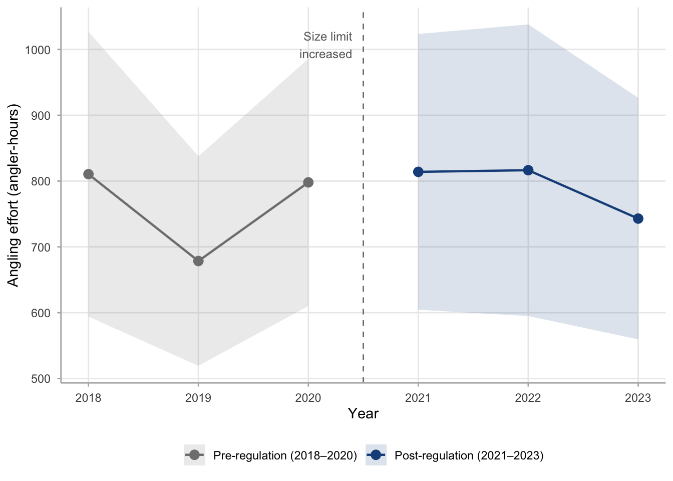
Figure 31.1 shows estimated angling effort for each year from 2018 to 2023, with 95% confidence intervals. The vertical dashed line marks the 2021 regulation change.
Figure 31.1: Annual angling effort at Harlan Reservoir, 2018–2023, with 95% confidence intervals. Pre-regulation years (gray) and post-regulation years (blue) show overlapping ranges with no directional trend. Effort ranged from r round(min(harlan_annual$effort_est)) to r round(max(harlan_annual$effort_est)) angler-hours per season. The 2021 size-limit increase did not reduce angling participation at the reservoir.
Effort ranged from 678 angler-hours in 2019 to 816 angler-hours in 2022. No directional trend is apparent before or after the regulation change, and the confidence intervals in each year overlap substantially with every adjacent year. The 2021 and 2022 post-regulation seasons in fact produced the two highest effort estimates in the series, though that difference is well within sampling uncertainty. The working conclusion is that angling participation at Harlan Reservoir was not affected by the size-limit change — a prerequisite for interpreting changes in CPUE and harvest as reflecting changes in the fish population rather than changes in fishing pressure.
31.3 Walleye catch rates across the monitoring period
Catch rate — CPUE, expressed as fish per angler-hour — is the primary metric of Walleye abundance and vulnerability to angling. Under a minimum size-limit increase, CPUE is expected to follow a characteristic pattern: an initial decline in the transition year as fish that were previously legal size become sub-legal under the new minimum, followed by a recovery as those cohorts grow past the new threshold and become available again. The magnitude and timing of the recovery depend on growth rates, natural mortality, and recruitment — quantities that the creel survey itself cannot estimate but that the monitoring series can inform.
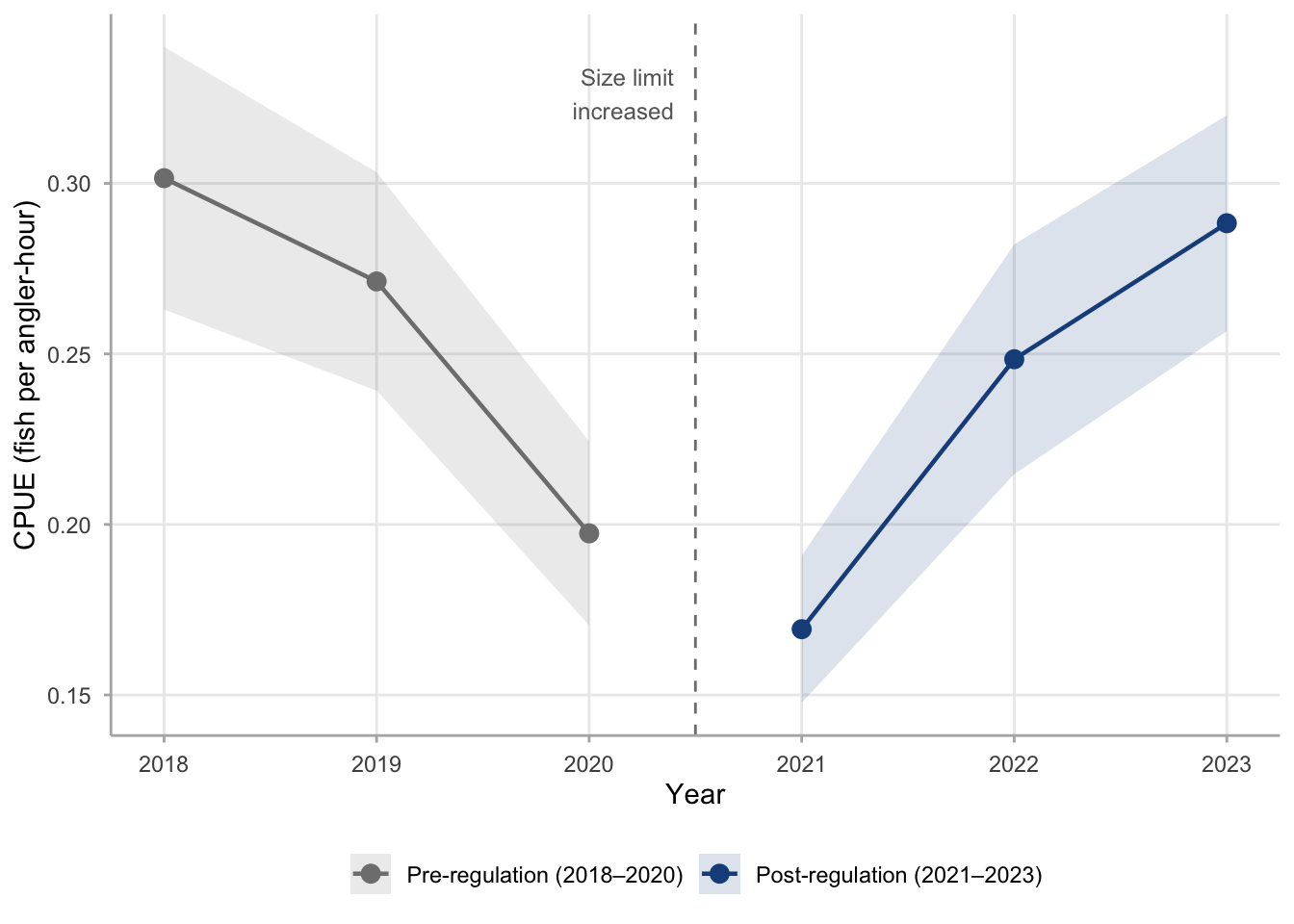
Figure 31.2 shows annual Walleye CPUE with 95% confidence intervals. The pre-regulation years exhibit a declining trend, with CPUE falling from 0.302 fish/hr in 2018 to 0.197 fish/hr in 2020. This decline predates the regulation change and suggests the fishery was already under sustained harvest pressure at the original 305 mm minimum — more fish were being removed annually than the population could replace.
Figure 31.2: Annual Walleye CPUE at Harlan Reservoir, 2018–2023, with 95% confidence intervals. Pre-regulation CPUE (gray) declined from 0.302 fish/hr in 2018 to 0.197 fish/hr in 2020. Following the 2021 size-limit increase (dashed line), CPUE reached its six-year low in the transition year before recovering to 0.288 fish/hr by 2023 — approaching the 2018 starting value.
The 2021 transition year produced the lowest CPUE in the series (0.169 fish/hr), consistent with the immediate contraction of the catchable pool following the size-limit increase. Fish in the 305–380 mm range — previously legal and thus catchable by harvest-oriented anglers — became catch-and-release only in 2021, effectively removing a cohort from the harvest-available fraction of the population without immediately replacing it. By 2022, CPUE had recovered to 0.248 fish/hr, and by 2023 to 0.288 fish/hr. The 2022 estimate from the access-point case study (Section 30.10) — produced by the full single-year pipeline — falls directly on this trajectory, confirming that the 2022 access-point survey results are consistent with the broader monitoring trend.
31.4 Walleye harvest trends
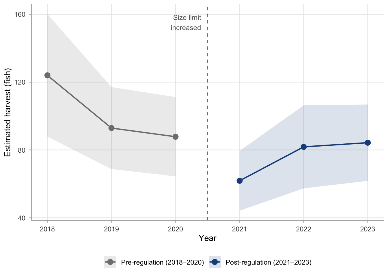
Where CPUE measures the catchable abundance visible to anglers, estimated harvest measures the actual number of fish removed from the population each season. For a size-limit regulation to produce a population-level benefit, harvest must decline. Figure 31.3 shows the six-year harvest trajectory.
Figure 31.3: Annual estimated Walleye harvest at Harlan Reservoir, 2018–2023, with 95% confidence intervals. Harvest declined steadily from 124 fish in 2018 to 88 fish in 2020 under pre-regulation conditions, then dropped sharply to 62 fish in 2021 — the first year under the 381 mm minimum size limit. Harvest recovered partially to 82–84 fish per season in 2022–2023, remaining well below pre-regulation levels.
Estimated harvest fell from 124 fish in 2018 — the monitoring period’s peak — to 62 fish in 2021, a reduction of 50% from the pre-regulation high. Harvest had already been declining modestly in 2019 and 2020 — consistent with the CPUE decline in those years suggesting a population under pressure — and the regulation accelerated that reduction sharply. Post-regulation harvests of 82 and 84 fish in 2022 and 2023, respectively, represent a partial recovery from the 2021 low but remain 24% below the pre-regulation weighted mean. Fish that previously would have been retained at 305–380 mm are now being released, keeping more individuals in the population to grow toward the 381 mm minimum and eventually beyond.
31.5 Before-after statistical contrast
Visual inspection of the time series is useful for identifying patterns, but it cannot distinguish a real change from sampling noise. The before-after statistical contrast described in Section 28.5 addresses this by computing precision-weighted means for each period and testing whether the difference between periods is significantly different from zero. Years with tighter confidence intervals receive more weight in the period mean than years with wider intervals.
with period standard error \text{SE}(\bar{y}_w) = 1 / \sqrt{\sum_t w_t}. Because the two periods are based on independent samples, the standard error of the difference is \text{SE}(\hat{\delta}) = \sqrt{\text{SE}_\text{before}^2 + \text{SE}_\text{after}^2}, and a z-test follows directly.
Table 31.2: Before-after statistical contrast for Walleye CPUE and estimated harvest at Harlan Reservoir. Precision-weighted means are computed for the pre-regulation period (2018–2020) and post-regulation period (2021–2023). The z-statistic and two-sided p-value test whether the difference between periods is distinguishable from zero. Both metrics changed significantly.
Metric
Before
After
Change
SE
z
p
CPUE (fish/hr)
0.244
0.216
-0.028
0.012
-2.31
0.0210
Harvest (fish)
96.300
73.200
-23.100
9.900
-2.33
0.0197
The precision-weighted mean CPUE was 0.244 fish/hr in the pre-regulation period and 0.216 fish/hr post-regulation (z = -2.31, p = 0.021). The precision-weighted mean harvest was 96.3 fish pre-regulation and 73.2 fish post-regulation (z = -2.33, p = 0.0197). Both differences are statistically significant.
The direction of the CPUE change — negative — may appear to contradict a regulation intended to increase Walleye abundance. However, this contrast includes the 2021 transition year, when the catchable pool contracted immediately as previously legal fish became sub-legal under the new minimum. The before-after contrast is the correct tool for answering “did anything change?” but a piecewise trend model (see Section 31.7) is better suited to separating the transition year’s contraction from the subsequent recovery.
31.6 Monitoring program precision: is the design stable?
Cross-year comparisons are only valid if the survey designs in each year are sufficiently consistent to produce comparable estimates. A year with anomalously low sampling coverage or high within-stratum variance will produce wide confidence intervals, which the precision-weighted analysis will down-weight — but it is still important to verify that no single year is so different in design quality that comparisons are compromised.
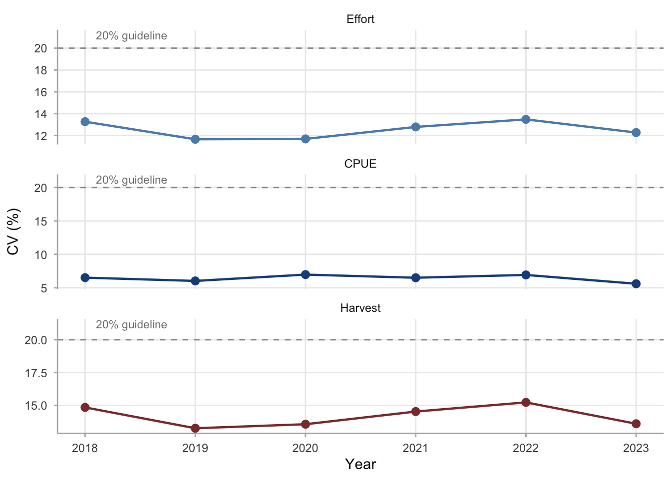
The coefficient of variation (CV) for each metric summarizes annual design precision in a scale-independent way. A stable CV across years indicates that sampling quality was consistent; a large CV in one year flags that year as a potential outlier worth investigating.
Figure 31.4: Annual coefficient of variation (CV, %) for effort, CPUE, and harvest at Harlan Reservoir, 2018–2023. All three metrics remain below the 20% precision guideline in every year, indicating consistent design quality across the monitoring period. Harvest carries the highest CV because it compounds variance from both the effort estimate and the per-trip harvest rate.
All three metrics maintained CVs below 20% in every year of the monitoring period — the conventional upper threshold for management-grade estimates. CPUE CVs were the lowest of the three (5.6 to 7%), reflecting the ratio estimator’s efficiency when catch rates are relatively stable within strata. Effort CVs ranged from 11.7 to 13.5%, and harvest CVs — the highest of the three — ranged from 13.3 to 15.2%. The absence of any outlier year confirms that the precision-weighted comparisons in this chapter are supported by consistently reliable design quality.
31.7 Piecewise trend: separating transition from recovery
The before-after contrast established that CPUE and harvest both changed significantly across the 2021 regulation. What it cannot show is whether the post-regulation period represents sustained decline or, as hypothesized, an initial transition dip followed by recovery. A piecewise weighted linear model — fitting separate slopes for the pre- and post-regulation periods — addresses this directly. The method is covered in Section 28.7; here it is applied to CPUE to characterize the direction of change within each period.
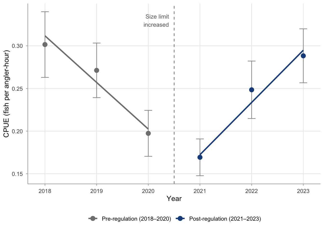
Figure 31.5: Piecewise weighted linear trend in Walleye CPUE at Harlan Reservoir, with separate slopes fitted for pre-regulation (gray) and post-regulation (blue) periods. The pre-regulation slope is r round(slope_before, 4) fish/hr/yr (declining), consistent with sustained overharvest under the 305 mm minimum. The post-regulation slope is r round(slope_after, 4) fish/hr/yr (recovering), indicating a directional reversal following the 2021 size-limit increase.
The pre-regulation slope is -0.0547 fish/hr/yr — a declining trend of approximately 5.5 fish per hundred angler-hours per year under the 305 mm minimum. The post-regulation slope is 0.0613 fish/hr/yr — a recovering trajectory of approximately 6.1 fish per hundred angler-hours per year. The sign reversal — from negative to positive — is the key qualitative finding. CPUE was declining under the previous size limit and has been recovering since the change. Whether either individual slope is statistically distinguishable from zero is less important than their directional consistency with the biological hypothesis: protected cohorts accumulating in the 305–380 mm range are growing toward the 381 mm minimum and beginning to appear in completed-trip interviews as legal catches.
It is worth noting the limits of three-year slopes. With only three data points per period, the piecewise model cannot reliably estimate nonlinear patterns within each period, and the interaction test for different slopes has low statistical power. The slopes here should be interpreted as summaries of direction, not precise rates of change. Extending the monitoring series through 2024 and 2025 will substantially improve the power to detect whether the post-regulation recovery trajectory is sustained or whether it plateaus.
31.8 Management interpretation
The six-year monitoring record supports three findings, each with a direct management implication.
Angling effort is stable. Effort estimates fluctuated around 777 angler-hours per season with no directional trend before or after the 2021 regulation. This matters because it rules out the most common alternative explanation for changes in CPUE and harvest: that anglers shifted their behavior in response to the rule change. The same amount of fishing is occurring; what changed is the fish population and the composition of the catch.
Harvest decreased substantially and has remained lower post-regulation. Estimated harvest fell roughly 24% from the pre-regulation weighted mean (96.3 fish) to the post-regulation weighted mean (73.2 fish). This reduction is statistically significant and biologically meaningful. Fish that were previously retained at 305–380 mm are now being released under the new minimum, contributing to the protected cohort growing toward 381 mm. The partial harvest recovery in 2022–2023 is consistent with some of those larger fish becoming legal as they grow past the 381 mm threshold.
CPUE declined in the transition year but has been recovering. The piecewise model shows a positive post-regulation slope, and by 2023 CPUE had returned to 0.288 fish/hr — close to the 2018 starting value of 0.302 fish/hr before the decline began. The before-after contrast shows a statistically significant reduction in the weighted mean CPUE across periods, driven largely by the 2021 transition year. Whether the recovery observed in 2022–2023 will continue to improve and eventually exceed pre-decline levels will depend on the year-class strength of fish now in the 305–380 mm range, which cannot be estimated from catch rates alone.
The monitoring program’s immediate recommendation is to continue the survey at the current design and precision for at least two additional years. The current design achieves CPUE CVs of approximately 6–7% and harvest CVs of 13–15%. At those precision levels, the survey can detect changes of roughly 20–30% in CPUE between adjacent years at 80% power. A continued recovery of 10–15% per year will not be distinguishable in any single year comparison but will be clearly visible in the accumulated series by 2025. Changing the survey design now would break the comparability that makes the before-after contrast valid.
31.9 Takeaway
This case study illustrates the monitoring application of creel surveys: using a consistent access-point design across multiple years to generate annually comparable estimates, then applying formal statistical methods to evaluate whether a management action has produced its intended outcome.
At Harlan Reservoir, six years of systematic monitoring show that a Walleye minimum size-limit increase in 2021 coincided with a statistically significant decline in estimated harvest, a temporary contraction of CPUE in the transition year, and a subsequent CPUE recovery trajectory consistent with the protected cohort growing toward the new minimum. Angling effort remained stable throughout, confirming that the changes in CPUE and harvest reflect population dynamics rather than shifts in angler behavior.
From a workflow standpoint, this chapter connects three elements: the single-year pipeline from the access-point case study (Section 30.10), where the 2022 estimates sit on the same trajectory as the monitoring series; the method introductions from Section 28.1 through Section 28.10; and the management context that motivates the analysis. The distinction between a methods chapter and a case study chapter is emphasis: here the goal is to answer a specific management question — did the regulation work? — rather than to demonstrate how the methods operate.
Key workflow steps for a multi-year monitoring case study:
Load pre-computed annual estimates rather than re-running individual year pipelines for every analysis
Inspect the full time series visually before fitting any statistical models — the plots in this chapter would have flagged a data problem in any single year
Confirm that design precision is consistent across years before comparing estimates; a year with an outlying CV should be investigated before being included in a weighted contrast
Apply a precision-weighted before-after contrast rather than an unweighted t-test; years with tight confidence intervals carry more information and should contribute more to the period mean
Use a piecewise model to separate the regulation transition year from the subsequent recovery; a single pre-versus-post contrast cannot distinguish these two phases
Report all three metrics — effort, CPUE, and harvest — together; no single metric tells the full story of a fishery’s response to regulation
Maintain the same survey design across years; changing stratification, shift structure, or sampling intensity resets the comparability baseline and undermines the monitoring program’s core value
Communicate the uncertainty alongside every point estimate to managers; a change that “looks big” in a bar chart may not be statistically detectable, and a monitoring program is only useful if decision-makers trust its precision