creel survey, fisheries, design-based inference, R, tidycreel, Quarto
6.1 Purpose
Chapter 1 named the five core estimands of a creel survey — effort, total catch, total harvest, total release, and catch rate — and described what each measures in general terms. That introduction was sufficient for motivating why creel surveys exist. It is not sufficient for analyzing creel data.
Estimation requires precision. The same English word — “catch,” “effort,” “angler” — conceals choices about units of measurement that propagate silently through every calculation. A catch rate computed from party-level data cannot be multiplied against effort estimated from individual-level counts without introducing bias. An estimate labeled “seasonal harvest” computed over a sampling frame covering only weekdays does not represent the full season. These errors are invisible unless the estimand, the unit, and the reporting domain are stated explicitly before the first calculation.
This chapter formalizes what Chapter 1 introduced. It defines the notation used throughout this book, explains the unit decisions that must be made before data collection begins, and introduces the concept of the reporting domain — the population of fishing events over which an estimate is claimed to apply.
This chapter covers:
formal definitions and notation for all five estimands;
units of measurement and why party-level and individual-level quantities cannot be interchanged;
why instantaneous and progressive counts estimate effort in hours, not trips;
reporting domains — temporal, spatial, species, and gear — and how they bound the scope of inference;
the problem of species-targeted effort and why certain domain-estimand combinations are undefined; and
how domain structure appears in the tidycreel data tables.
6.2 The five estimands, formally
Every creel survey produces estimates of some subset of five population quantities. These quantities exist at two levels: the individual observation level, recorded during a single interview or count, and the population level, the aggregate across all fishing activity during the target period. Population-level quantities are the targets of inference; individual-level quantities are what the estimators use as inputs.
Table 6.1 defines the notation used throughout this book.
Table 6.1: Notation used throughout this book. Individual-level quantities are collected in the field; population-level quantities are the targets of inference. Subscripts s, i, and k denote stratum, sampled day, and interview party when stratified estimators are developed in later chapters.
Symbol
Definition
Level
Units
e_k
Fishing time for party k
Interview
angler-hours
h_k
Fish harvested by party k
Interview
fish
c_k
Fish caught (harvested + released) by party k
Interview
fish
r_k
Fish released by party k
Interview
fish
x_i
Anglers counted during count i
Count
anglers
E
Total effort: total fishing time by all parties during the target period
Population
angler-hours
C
Total catch: all fish encountered by all anglers during the target period
Population
fish
H
Total harvest: fish retained by all anglers during the target period
Population
fish
R
Total release: fish returned by all anglers during the target period
Population
fish
\widehat{\text{cpue}}
Catch per unit effort: ratio of total catch to total effort
Population
fish per angler-hour
\hat{E}, \hat{C}, \hat{H}, \hat{R}
Sample estimates of population quantities
—
same as above
Effort
Effort (E) is the total fishing time expended by all anglers at a waterbody or site during the target period, expressed in angler-hours. It is the foundational estimand: it appears in the denominator of catch rate, serves as the multiplier that scales catch-rate estimates up to total catch, and is the primary measure of recreational pressure used by managers to track how intensively a fishery is used. Getting E wrong contaminates every downstream estimate.
Effort is derived from counts, not from interviews. An instantaneous count records how many anglers are present at a moment in time; that observation, together with the length of the sampling period and the relevant trip-duration information, enters an estimator of angler-hours. Interviews provide catch and fishing time per party, which enter the catch-rate calculation but not the effort estimate directly. This separation of sources is structural and intentional, and is explained in Section 6.4.
Total catch and its components
Total catch (C) is the number of fish encountered — meaning hooked and brought to hand — by all anglers during the target period, regardless of whether fish were retained or returned. It is the sum of harvest and release:
C = H + R
This additive relationship is definitional. If C, H, and R are estimated from the same data using the same estimator, they are additively consistent by construction. If each is estimated from a different subset of the interview records — for example, harvest from completed-trip interviews only and total catch from all interviews — the three estimates may not add up correctly. Section 6.8 returns to this point.
Total harvest (H) is the catch component most directly linked to population dynamics and management action. Bag limits, size limits, and season dates act on harvest. Exploitation rate uses harvest as its numerator. In most agency creel programs, harvest is the primary estimand.
Total release (R) is the catch component returned to the water. Its importance depends on the fishery. In trophy or catch-and-release waters, R may exceed H substantially and is needed to estimate release mortality. In put-and-take stocking programs, R is low and harvest is the primary focus.
Catch rate
Catch rate (\widehat{\text{cpue}}) is the ratio of total catch to total effort:
\widehat{\text{cpue}} = \frac{\hat{C}}{\hat{E}}
expressed in fish per angler-hour. It is the most widely tracked creel diagnostic for changes in fish availability, because it can be compared across years without requiring equal sampling intensity as long as the design is consistent.
Interpreting a catch rate trend requires understanding what drives changes in the ratio. A declining rate can reflect a declining fish population, a change in how anglers distribute effort spatially, a change in gear, or a shift in target species composition. Catch rate is a symptom; its diagnosis requires additional context about the fishery.
Important
Catch rate (\widehat{\text{cpue}}), harvest rate (\hat{H}/\hat{E}), and release rate (\hat{R}/\hat{E}) are different quantities. A catch rate of 0.5 fish per angler-hour means anglers on average encountered 0.5 fish per hour regardless of whether fish were kept or returned. Report harvest rate and release rate from the appropriate numerator when both components are of interest.
Secondary estimands
The five core estimands — effort, total catch, total harvest, total release, and catch rate — are the primary targets of most creel surveys. Several secondary quantities are frequently reported alongside them. They are derived from the same field records but answer different management questions.
Trip success rate is the proportion of completed angler-trips that resulted in at least one fish of the target species being caught. It is an angler-experience metric rather than a population-dynamics metric: a fishery can have a low trip success rate but high total harvest if the successful trips are extremely productive. Conversely, high trip success with low total catch indicates that many anglers are catching exactly one fish and not much more. Trip success rate is computed directly from the interview stream without reference to the count-based effort estimate.
Harvest rate is the proportion of caught fish that were retained: \hat{H}/\hat{C}. A declining harvest rate over time on a catch-and-release regulation may indicate angler compliance; a suddenly high harvest rate may indicate unregulated sites or non-compliance with bag limits. Harvest rate can be computed at the species level from the catch table.
Party size distribution describes the frequency distribution of the number of anglers per party. This is not usually a management target but is needed for converting party-level quantities to individual-level quantities correctly. If mean party size is used in a conversion, the conversion is biased when party size and fishing duration are correlated (as shown in Section 6.3). Retaining the full distribution avoids this problem.
Length-class harvest is harvest partitioned into length categories — often regulatory length classes such as “sublegal,” “slot limit,” and “trophy.” This is derived by joining interview harvest counts to biological data (lengths measured from harvested fish brought to the ramp) and assigning each fish to a length class. The biological data chapter in Part V covers this estimand in full using est_length_distribution() and est_compliance(). It is particularly important in slot-limit regulations where harvest of fish within the slot is prohibited.
Angler-days is total effort expressed as angler-days (complete eight- or ten-hour outings) rather than angler-hours. It is used mainly for access capacity planning and is computed from the same count-based effort framework with a different time unit. Because “angler-day” is an ambiguous unit (does it mean 8, 10, or 12 hours?), statements using it should always define the denominator.
6.3 Units of measurement
The notation in Table 6.1 assigns angler-hours as the unit of effort and fish per angler-hour as the unit of catch rate. These are not the only possibilities. Creel clerks may record fishing time per party, per individual, or as a categorical trip duration; counts may enumerate parties rather than individuals; reporting may use trips instead of hours. Each choice leads to a different unit of effort and a different set of valid calculations. Mixing units across steps produces bias that is invisible in the output unless the computation is traced carefully (Pope et al. in press).
The experimental unit: party or individual
The first unit decision is the experimental unit — the entity at which interview information is collected.
Party-level collection treats the fishing party (the group that travels and fishes together) as the unit. One record per group: number of anglers in the party, total fishing time for the group, total catch, and retention decisions. Most access-point creel programs in North America use party-level collection because parties arrive and depart together, and one interview per group is operationally faster than one per person (Malvestuto 1996).
Individual-level collection records each angler separately, providing higher resolution on within-party heterogeneity but requiring more time and producing incomplete records when party members have different arrival and departure times.
The choice must be made before data collection begins, stated in the survey protocol, and maintained consistently from field entry through final estimation. Changing levels midstream, or converting between levels after collection, introduces bias whenever party size and fishing duration are correlated. The following example, adapted from Pope et al. (in press), illustrates why.
Note
The unit conversion problem
Four parties were interviewed on a single day at a small impoundment:
If the clerk recorded party-level fishing time — 4, 4, 4, and 12 hours per party — the mean party duration is 6 hours and the mean party size is 2 anglers. An analyst who multiplies these means to convert party-hours to angler-hours gets 6 \times 2 = 12 angler-hours per party, or 4 \times 12 = 48 total — not 40. The units appear to cancel (\text{hours/party} \times \text{anglers/party}) but the arithmetic does not work, because the mean of a product is not the product of the means when duration and party size are correlated. Party D (one angler, 12 hours) pulls the duration mean up while contributing only one angler to the size mean.
If instead the clerk had collected individual-level records, the mean individual duration would be 40/8 = 5 hours, and total effort would be 8 \times 5 = 40 angler-hours — correct.
The same problem arises in reverse: converting an individual-level estimate to party level produces a mean party duration of 5 hours, while the true average is 6 hours.
The only remedy is to define the experimental unit before collection and compute all quantities at that level consistently. Conversion is not safe as a post-hoc adjustment.
Effort unit: hours or trips
The second unit decision is whether to express effort in angler-hours or angler-trips.
Angler-hours measure time on the water. An angler who fishes for two hours contributes twice as much effort as one who fishes for one hour. Hours are the natural denominator when fish encounter rates are assumed to be proportional to fishing time.
Angler-trips count discrete outings regardless of duration. Two parties with the same trip count but very different durations contribute equally. Trips are appropriate when the management question is about the number of angling events — relevant for access planning, crowding studies, or trip-success analysis — rather than total time on the water.
All estimators in this book use angler-hours as the primary effort unit. This is consistent with the count-based effort estimators described in Section 6.4, which yield angler-hours directly, and with interpreting catch rate as a per-unit-time encounter rate.
6.4 Why counts estimate effort, not trips
Effort in a creel survey is estimated from counts, not from interviews. This architectural choice has a direct implication for units: count-based effort estimators produce angler-hours, not angler-trips (Hoenig et al. 1993).
An instantaneous count records the number of anglers present at a randomly chosen moment during the sampling shift. The expected value of that count is proportional to the total angler-hours expended during the shift — not to the number of trips. An angler who fishes for eight hours is present in the system for eight times as long as one who fishes for one hour, and is therefore eight times more likely to be observed at a random moment. The count is an area-under-the-curve measure of time on the water.
To see this formally, suppose N anglers each fish for e_j hours during a sampling shift of duration T. If counts are conducted at randomly chosen moments within the shift, the expected count at any moment is:
where E = \sum_{j=1}^N e_j is total angler-hours. Rearranging:
\hat{E} = x \times T
This is the instantaneous count estimator: observed anglers times shift duration equals estimated angler-hours. The number of trips does not appear in the estimator and cannot be recovered from it.
The practical consequence is that catch rates derived from count-based effort are in fish per angler-hour. Multiplying a per-hour catch rate by an hour-based effort estimate yields total catch with internally consistent units. An analyst who wants to report catch rates in fish per trip must obtain the number of trips from the interview stream and verify that the interview sample represents all trips — not all angler-hours — which requires a different sampling condition.
In plain language, counts answer “how long was the fishery active?” and interviews answer “what happened during that activity?” The first is a time total; the second is a trip summary. They are related, but they are not interchangeable.
Unit decisions in practice
When setting up a new creel program, the unit decisions above should appear explicitly in the field data entry form and the data dictionary, not just in the analysis protocol. Common practices that create unit ambiguity in legacy datasets:
“Trip hours” without specifying party or individual. If the form says “hours fished” and three crew members collected data, it is often unclear whether hours were recorded for the whole party or per person. Resolving this ambiguity retrospectively requires re-contacting field clerks or using internal consistency checks (e.g., does party_size × hours match the total hours recorded?).
Party size absent from the interview record. Without party size, it is impossible to convert party-level catch to individual-level catch or to detect whether a high catch record reflects one prolific angler or a group of anglers. All interview records should include n_anglers.
Mixed units across sections or years. Some programs shift from party-level to individual-level recording between field seasons without updating the analysis code. The resulting dataset is a mixture of units with no field identifying which record uses which convention. This is one of the most difficult data quality problems to diagnose post hoc.
The validate_creel_data() function in tidycreel checks for these conditions and returns a structured report with any flagged inconsistencies. It should be run on every season’s data before estimation begins.
── Creel Data Validation ───────────────────────────────────────────────────────
63 pass | 0 warn | 0 fail
── Table: counts ──
✔ reservoir
✔ type: class: character
✔ na_rate: 0 / 236 NA (0%)
✔ empty_strings: none
✔ date
✔ type: class: Date
✔ na_rate: 0 / 236 NA (0%)
✔ date_range: all within 1970-01-01 - 2100-12-31
✔ day_type
✔ type: class: character
✔ na_rate: 0 / 236 NA (0%)
✔ empty_strings: none
✔ period
✔ type: class: numeric
✔ na_rate: 0 / 236 NA (0%)
✔ negative_values: none
✔ section
✔ type: class: character
✔ na_rate: 0 / 236 NA (0%)
✔ empty_strings: none
✔ count_time
✔ type: class: character
✔ na_rate: 0 / 236 NA (0%)
✔ empty_strings: none
✔ bank_anglers
✔ type: class: integer
✔ na_rate: 0 / 236 NA (0%)
✔ negative_values: none
✔ angler_boats
✔ type: class: integer
✔ na_rate: 0 / 236 NA (0%)
✔ negative_values: none
✔ boat_anglers
✔ type: class: integer
✔ na_rate: 0 / 236 NA (0%)
✔ negative_values: none
── Table: interviews ──
✔ reservoir
✔ type: class: character
✔ na_rate: 0 / 600 NA (0%)
✔ empty_strings: none
✔ date
✔ type: class: Date
✔ na_rate: 0 / 600 NA (0%)
✔ date_range: all within 1970-01-01 - 2100-12-31
✔ day_type
✔ type: class: character
✔ na_rate: 0 / 600 NA (0%)
✔ empty_strings: none
✔ period
✔ type: class: numeric
✔ na_rate: 0 / 600 NA (0%)
✔ negative_values: none
✔ section
✔ type: class: character
✔ na_rate: 0 / 600 NA (0%)
✔ empty_strings: none
✔ interview_id
✔ type: class: integer
✔ na_rate: 0 / 600 NA (0%)
✔ negative_values: none
✔ party_id
✔ type: class: character
✔ na_rate: 0 / 600 NA (0%)
✔ empty_strings: none
✔ n_anglers
✔ type: class: numeric
✔ na_rate: 0 / 600 NA (0%)
✔ negative_values: none
✔ angler_type
✔ type: class: character
✔ na_rate: 0 / 600 NA (0%)
✔ empty_strings: none
✔ angler_method
✔ type: class: character
✔ na_rate: 0 / 600 NA (0%)
✔ empty_strings: none
✔ hours_fished
✔ type: class: numeric
✔ na_rate: 0 / 600 NA (0%)
✔ negative_values: none
✔ trip_status
✔ type: class: character
✔ na_rate: 0 / 600 NA (0%)
✔ empty_strings: none
The Harlan data passes all checks cleanly. A pass here means the unit decisions recorded in the data — party-level, angler-hours, consistent access-type coding — are internally consistent and the tables are ready for domain-restricted estimation. Chapter 9 covers the full validation battery and what to do when checks fail.
6.5 Reporting domains
An estimand without a domain is incomplete. “Total harvest” is undefined unless it specifies harvest of which species, by which anglers, at which locations, during which period. The reporting domain is the set of fishing events to which an estimate is claimed to apply.
Every creel survey operates within an overall sampling frame — the set of sites, dates, and access types covered by the design. The full-frame estimate corresponds to the broadest domain. Narrower estimates apply to domain-restricted subsets: harvest at one ramp only, walleye harvest only, harvest on weekend days only. Getting the domain right matters because domain-restricted estimates and full-frame estimates have different denominators, different subsets of interview records, and sometimes different estimation strategies.
The domain is part of the estimand, not just a label attached afterward. “Walleye harvest on weekend mornings in the north section” and “seasonal harvest across the full reservoir” are different questions, so they require different data cuts and different expectations for precision.
Four dimensions define the reporting domain in most creel surveys.
Temporal domains
Day type. Fishing pressure on weekends can be several times higher than on weekdays; holiday weekends can be higher still. The standard design stratifies days into at least two types — weekday and weekend — and treats each as a separate domain for sampling and estimation. Contemporary designs add a third stratum for high-use days where pressure may be an order of magnitude above typical weekends (Pope et al. in press; Malvestuto 1996). Aggregating across day types without stratification produces a biased seasonal estimate because sampled days are not a proportional cross-section of all days.
Shift. Many designs cover only part of the day in each sampled period. Shift-level estimates restrict the domain to that portion of the day; full-day estimates require extrapolating across shifts, which demands either that both shifts were sampled or that shift-level fishing intensity is assumed equal.
Month or season. Monthly estimates aggregate across day types within the month; seasonal estimates aggregate across months. A monthly total multiplies mean daily effort by the number of calendar days in the month; a seasonal total multiplies mean daily effort by the number of days in the full season. Applying a seasonal multiplier to compute a monthly total overstates harvest by the ratio of season to month length.
Year. Annual estimates combine monthly or seasonal estimates. Consistent year-to-year estimation requires the same strata definitions, domain boundaries, and unit choices in each year. Changes in any of these create apparent trends that are analytical artifacts rather than biological signals.
Spatial domains
Section. A named segment of the waterbody associated with a specific access site, boat ramp, or shoreline stretch, sampled independently. Section-level estimates use only the counts and interviews collected at that site.
Waterbody. An entire lake, reservoir, or river. Section estimates are summed to produce the waterbody total. If sections differ substantially in fishing pressure or fish assemblage, estimating each separately before summing reduces bias that would result from pooling heterogeneous access points (Pope et al. in press).
Region. Multiple waterbodies grouped for reporting. Regional estimates require that each waterbody was sampled with a design that supports waterbody-level inference, and that waterbodies were selected in a way that represents the region.
Cross-domain combinations and sample size decay
The four domain dimensions — temporal, spatial, species, access type — can be combined. A reporting request for “walleye harvest by boat anglers during June on the north section” is the intersection of all four domains simultaneously. Each intersection step reduces the sample size available for that estimate. If 600 interviews are collected over the season, and 40% are from boat anglers, and 25% are from June, and 30% are from the north section, and 60% involve any walleye catch, the intersection may contain only a handful of parties — far too few for a useful estimate.
This sample-size decay problem is not a failure of estimation theory; it is a fundamental constraint of domain-restricted inference. The statistical machinery works correctly on ten interviews, but the resulting confidence interval may span an order of magnitude. The practical response is to decide which domain dimensions are essential for the management question and which can be aggregated without misleading the user. A request for “walleye harvest by boat anglers” that arrives after data collection has already begun cannot be answered precisely if the original design did not power for it.
The book-level rule is to state the narrowest domain you actually need before the season starts, then treat everything broader or narrower as a secondary cut of the same data. That discipline is what keeps the estimate honest when the data become sparse.
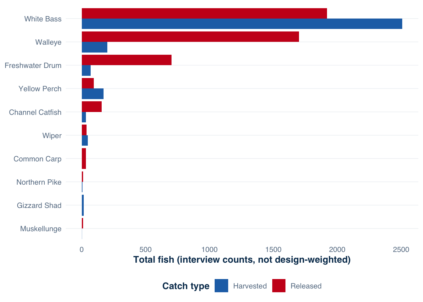
Figure 6.1 below shows the distribution of harvest and release counts across species and catch type in the Harlan dataset — the starting point for any species-domain restricted estimate.
Code
harlan_catch |>group_by(species, catch_type) |>summarise(n_fish =sum(n_fish), .groups ="drop") |>filter(n_fish >0) |>mutate(species =reorder(species, n_fish, sum)) |>ggplot(aes(x = n_fish, y = species, fill = catch_type)) +geom_col(position ="dodge") +scale_fill_manual(values =c(harvested ="#2171b5", released ="#cb181d"),labels =c(harvested ="Harvested", released ="Released") ) +labs(x ="Total fish (interview counts, not design-weighted)",y =NULL,fill ="Catch type" ) +theme_creel() +theme(legend.position ="bottom")
Figure 6.1: Total fish counted in interviews at Harlan Reservoir, by species and catch type. Walleye show the largest release counts relative to harvest, reflecting size-limit compliance and angler catch-and-release behavior for that species. These are raw interview totals, not design-weighted estimates.
Note that Figure 6.1 shows raw interview totals, not design-weighted population estimates. A species with a large raw harvest count in the interview sample may have a small design-weighted harvest estimate if its harvest was concentrated on a few high-activity days that happened to be sampled. The design-weighted estimates — computed in Chapter 4 — can differ substantially from these raw sums.
Species and gear domains
Species. An estimate can be restricted to a single target species or a species group. Species membership is determined at the interview: the catch table records which species were kept or released by each party. Species-domain estimates use only the subset of catch records for that species while retaining the full effort estimate — see Section 6.5.5 for why this matters.
Access type and gear. Estimates can be restricted to boat anglers, bank anglers, fly-fishing anglers, or bait users. Access type is frequently an important domain because boat and bank anglers target different areas of the waterbody, encounter different assemblages, and often have systematically different catch rates for the same species. When access type is distinguishable during counts — boat trailers in the parking lot vs. anglers on foot — effort can also be partitioned by access type, and it must be for the domain consistency rule in Section 6.8 to be satisfied.
In practical terms, access type is not just a label. It is a different fishing population with a different denominator, so a boat-angler rate only makes sense if the effort it is multiplied by also came from boat anglers.
The impossible domain: species-targeted effort
One domain restriction unavailable from instantaneous or progressive counts is species-targeted effort: total fishing time expended only by anglers targeting a particular species.
This would be a natural quantity to have — if you wanted a walleye catch rate specifically among walleye-targeting anglers, you would divide walleye catch by walleye-targeting effort. The problem is that counts cannot record which anglers are targeting which species. When a clerk counts 30 anglers on a reservoir, she cannot identify the walleye-targeting subset from those targeting bass or catfish. There is no count-derived denominator for species-specific effort.
An apparent workaround is to scale total effort by the fraction of interviewed anglers who reported targeting a species. If 35 percent of interviewed parties reported targeting walleye, one might use 0.35 \times \hat{E} as walleye-targeting effort. This requires assuming that the fraction of walleye-targeting anglers in the interview sample equals the fraction present in the system during counts — an assumption that fails whenever targeting behavior correlates with time of day, day type, or access type in ways not captured by the sampling design (Pope et al. in press).
The correct approach is to use total effort as the denominator for species-specific catch rates. A walleye catch rate of 0.2 fish per angler-hour means anglers on average caught 0.2 walleye per hour of total fishing time — not per hour of walleye-targeting time. This is interpretable: it represents the expected walleye catch per angler-hour from the full fishery. Comparing species-specific rates on this shared denominator is valid. Comparing rates computed on species-targeting denominators is not, because those denominators come from different, incomparable subsets of the fishing population.
The rule is simple: if counts cannot tell you who was targeting a species, they cannot supply species-targeting effort. The denominator has to stay at the level the counts can actually observe.
6.6 Interview-reported effort vs. count-estimated effort
The creel data tables contain two distinct effort signals: effort reported by anglers during interviews (hours_fished in harlan_interviews) and effort estimated from instantaneous counts (bank_anglers and boat_anglers in harlan_counts). These two quantities measure different things and should not be confused.
Interview-reported effort is the fishing duration self-reported by each angler party at the time of the interview. It is a party-level quantity in angler-hours, appropriate for computing catch rates (fish per angler-hour) from the interview sample. It is not a population-level estimate of effort. The interviewed parties are a sample of all parties that fished on the sampled day; summing or averaging their trip durations without design weighting does not produce a valid estimate of total effort for the day.
Count-estimated effort is derived from the instantaneous count observations in harlan_counts, scaled by shift duration. It is a population-level estimate of total angler-hours on the waterbody during the sampled period, with a variance that reflects between-day variability in the count data. This is the \hat{E} used in \hat{C} = \hat{r} \times \hat{E}.
These two signals serve different roles in the estimation pipeline. Interview-reported effort provides the denominator for catch rates: \hat{r} = \sum_k h_{k} / \sum_k e_{k}, where the sum is over interviewed parties. Count-estimated effort provides the multiplier that scales those rates to the fishery level: \hat{C} = \hat{r} \times \hat{E}.
However, comparing the two signals can serve as a useful diagnostic. If interview-reported total trip hours on a sampled day greatly exceed the count-estimated angler-hours for that day, it may indicate a counting error (too few counts, a short shift, or missed anglers). If count-based effort is much larger than interview totals would imply, the interview sample may be missing a substantial portion of the angling population — a potential non-contact or non-response bias.
Code
# Interview-side effort: total hours fished on sampled days, complete trips onlyinterview_effort_by_day <- harlan_interviews |>filter(trip_status =="complete") |>group_by(date) |>summarise(interview_angler_hours =sum(hours_fished * n_anglers),n_parties =n(),.groups ="drop" )# Count-side effort: sum of anglers counted, as a proxy for relative activitycount_activity_by_day <- harlan_counts |>group_by(date) |>summarise(total_counted =sum(angler_count),.groups ="drop" )# Join for comparisoneffort_compare <- interview_effort_by_day |>left_join(count_activity_by_day, by ="date")head(effort_compare)
These two columns are not directly comparable in magnitude — interview hours reflect only the interviewed subsample while count totals reflect instantaneous snapshots — but their correlation and relative patterns across sampled days provide a useful consistency check. Large outliers (days with high interview hours but low count activity, or vice versa) merit investigation of the field records.
6.7 Poststratification and domain assignment
For most spatial and temporal domains, membership is determined before the interview: a sampled day is either a weekday or a weekend; a section is north or south. These are pre-defined strata whose domain assignment is established by the sampling design.
Some domain restrictions can only be assigned after the interview. Bernard et al. (1998) give guided versus unguided anglers as an example: a clerk does not know whether an approaching angler is a guided client until the interview begins. This is poststratification — domain membership is assigned during data analysis, not during sampling.
Poststratification is valid when the probability of being assigned to a given poststrata does not depend on which days or times were sampled — that is, when the mix of guided and unguided anglers is approximately stable across the sampling schedule. When this holds, poststratified estimates have valid variances and the same unbiasedness properties as pre-stratified estimates. When it fails — for instance, if guided anglers predominantly fish on weekends and weekends were oversampled — poststrata estimates are biased.
Access type (boat vs. bank) is frequently treated as a poststrata when both types are present at the same sites and clerks cannot pre-assign arriving parties. The clerk records access type during the interview; estimates are computed separately for each type after the fact. If counts also distinguish boat and bank anglers independently, the poststratification is equivalent to pre-stratification for the effort calculation as well.
6.8 Cross-domain consistency
Total harvest is estimated by multiplying a catch rate by total effort: \hat{H} = \widehat{\text{hpue}} \times \hat{E}. This product is meaningful only when the rate and the effort apply to the same domain. If effort is estimated for all anglers at a waterbody but the catch rate comes from boat-angler interviews only, the product gives total boat-angler harvest a denominator drawn from all anglers. The result is neither a boat-angler total nor a waterbody total; it is a hybrid quantity with positive bias and no clear interpretation.
Important
Domain consistency rule. The effort domain and the catch-rate domain must be identical before multiplying them to produce a total catch or harvest estimate. If they differ, either restrict the effort estimate to match the catch-rate domain, or recompute the catch rate to cover the same domain as the effort.
Access-type partitioning. If counts distinguish boat and bank anglers — via boat trailers in the ramp lot and bank anglers on foot — effort can be partitioned by access type. In that case, compute boat catch rates from boat interviews, bank catch rates from bank interviews, then multiply each by the corresponding access-type effort, and sum the two totals for the waterbody estimate. Multiplying boat catch rates by total effort conflates the two populations.
Species partitioning. Species-specific effort cannot be extracted from counts (Section 6.5.5), so use total effort as the denominator for species-specific rates. Total harvest of species s is:
where \widehat{\text{hpue}}_s is harvest of species s per angler-hour of total effort and \hat{E} is total angler-hours. Both share the same denominator, so the domains are consistent. Summing \hat{H}_s across all species should reproduce \hat{H}, which provides a useful consistency check.
The additive identity \hat{C} = \hat{H} + \hat{R} should also hold when catch, harvest, and release are estimated from the same interview records. If any of the three uses a different subset, verify additivity before reporting.
6.9 The domain-estimand combination
Every creel estimate is a specific combination of an estimand and a domain. Writing this combination explicitly before analysis is the most useful discipline in creel survey work. A complete specification looks like:
“Total harvest of largemouth bass by boat anglers during June–August at Lake X, expressed in angler-hours using party-level interview data.”
This statement specifies: estimand (total harvest), species domain (largemouth bass), access-type domain (boat anglers), temporal domain (June–August), spatial domain (Lake X), and units (angler-hours, party-level). Every subsequent calculation is either consistent with this specification or it is in error.
Table 6.2 gives examples of how domain and estimand combine to produce specific claims with defined denominators.
Table 6.2: Domain and estimand combinations produce specific inferential claims with defined denominators. Mixing domains between numerator and denominator — catch rate from boat anglers divided by total effort — invalidates the estimate.
Estimand
Temporal
Spatial
Species
Unit
Denominator
Total harvest
Season
Waterbody
All species
Angler-hours
N_s \times \bar{E}_s summed over strata
Total catch
Month
Section
Largemouth bass
Angler-hours
Days in month \times mean daily effort at section
Catch rate
Season
Waterbody
Walleye
Fish/angler-hour
Total effort (all species)
Total effort
Weekend days
Waterbody
N/A
Angler-hours
Number of weekend days \times mean weekend effort
Total release
Season
Boat anglers
All species
Angler-hours
Boat-angler effort only
6.10 Domain structure in tidycreel
In tidycreel, reporting domains are represented as columns in the data tables that flow through the estimation functions. Each interview record carries the fields that define its domain membership — the sampled day (temporal), the section (spatial), angler type (access type), and catch species (species). Estimation functions use these columns as grouping variables to compute domain-restricted estimates.
The Harlan Reservoir dataset illustrates this structure. After loading the four tables:
Code
harlan_schedule <-readRDS(here("data/harlan_schedule.rds"))harlan_counts <-readRDS(here("data/harlan_counts.rds"))harlan_interviews <-readRDS(here("data/harlan_interviews.rds"))harlan_catch <-readRDS(here("data/harlan_catch.rds"))# Bank anglers are counted directly; boats are counted and expanded by the# mean anglers per boat party measured in the interviews.harlan_counts <-derive_angler_count( harlan_counts,bank = bank_anglers,boat_count = angler_boats,party_size =mean_party_size(harlan_interviews, n_anglers, angler_type = angler_type))
The harlan_interviews table carries all temporal, spatial, and access-type domain fields alongside the effort recorded for each party:
Each column encodes a domain dimension: date and day_type give the temporal domain, section gives the spatial domain, and angler_type (boat vs. bank) gives the access-type domain. The period column indicates which part of the day (morning vs. afternoon shift) the interview occurred in — relevant when shift-level domain estimates are needed. The interview_id is the key that links interview records to catch records.
The harlan_catch table carries the species domain. Each row records the number of fish of one species, of one catch type (harvested or released), for one party:
Code
head(harlan_catch)
# A tibble: 6 × 4
  interview_id species         catch_type n_fish
         <int> <chr>           <chr>       <int>
1            1 White Bass      released       11
2            1 White Bass      harvested      32
3            1 Yellow Perch    released        1
4            1 Walleye         released        0
5            4 White Bass      harvested       9
6            4 Freshwater Drum released        3
The linkage between tables is one-to-many through interview_id: one interview party in harlan_interviews may correspond to multiple rows in harlan_catch — one per species per catch type encountered. Parties that caught nothing of a given species have no row in harlan_catch for that species; absence is implicit, not represented by a zero row. This matters when computing species-specific catch rates across the full interview sample: the denominator must count all interviewed parties (including those with zero catch of the target species), not just those present in the catch table.
Demonstrating domain structure: walleye harvest by angler type
To make the domain concepts concrete, consider computing total Walleye harvest separately for boat and bank anglers — a domain-restricted estimate combining the species domain (Walleye) and the access-type domain (boat vs. bank).
Step 1: Extract Walleye harvest per party from the catch table.
Step 3: Compute harvest rates (fish per angler-hour) separately by access type. This is an interview-only summary — it will be multiplied by effort estimates in Chapter 4 to produce domain-consistent totals.
The harvest rates from Step 3 must be multiplied by access-type-specific effort estimates — boat-angler effort for the boat rate, bank-angler effort for the bank rate — not by total effort. If boat-angler effort is unavailable because counts did not distinguish boat and bank anglers, the correct response is to combine the two access types into a single domain rather than multiply a boat-only rate by total effort. This is the domain consistency rule applied to a concrete case.
Note
This manual version stays visible here so the domain logic is easy to follow. In practice, estimate_total_harvest() handles the join, zero-filling, and rate computation internally, and estimate_effort() supplies the effort denominator from the count table. The underlying arithmetic is identical; only the interface changes. Chapter 4 replaces this manual pipeline with the full function workflow.
6.11 Visualizing domain structure
Domain structure is not just an abstract design concept — it is visible in the data. Plotting summary statistics by domain dimension reveals whether domains differ in ways that require separate estimation or whether pooling is defensible.
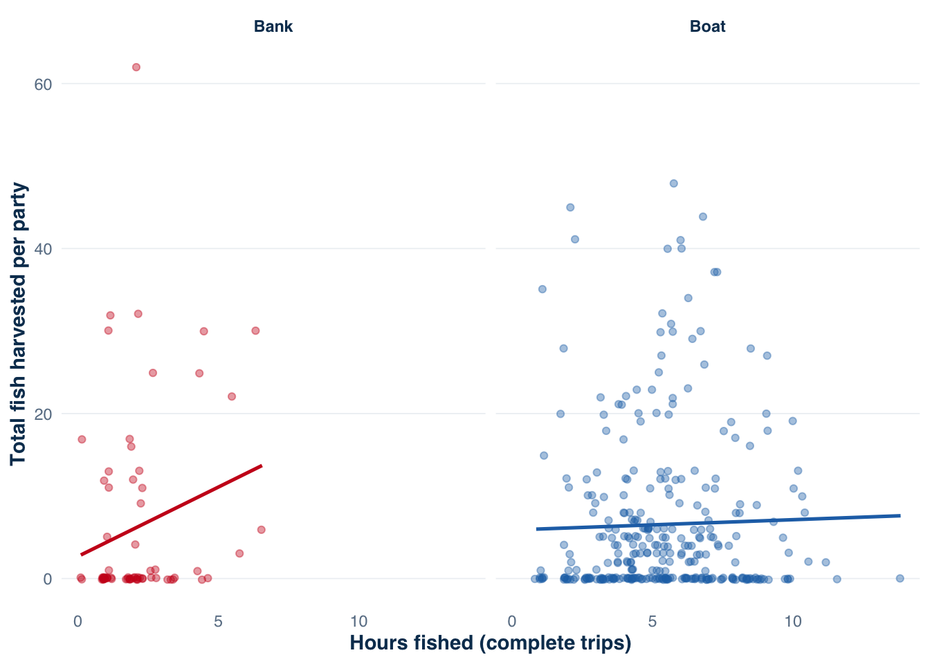
Figure 6.2 shows the distribution of trip duration (hours fished) and the number of fish harvested per party, split by angler type at Harlan Reservoir. Both dimensions of domain structure — effort expended and catch produced — differ between boat and bank anglers.
Figure 6.2: Trip duration and total harvested fish per party at Harlan Reservoir, by angler type (completed trips only). Differences in both effort expended and harvest per trip justify treating boat and bank anglers as separate domains in estimation.
Figure 6.2 makes two things clear. First, boat anglers fish longer trips on average than bank anglers. Second, harvest per party increases with hours fished in both access types, but the slopes and intercepts differ. A single harvest-rate (fish per angler-hour) computed from pooled boat and bank interviews would sit between the two access-type rates, representing neither accurately. The domain consistency rule requires that when effort can be partitioned by access type — which it can at Harlan, because harlan_counts records boat and bank anglers separately — the harvest rate must also be partitioned.
Domain imbalance and its consequences
Domain-restricted estimates have smaller sample sizes than full-frame estimates. This is unavoidable: splitting 600 interview parties into boat and bank subsets produces two smaller groups, each with a wider confidence interval than the pooled estimate. There is no statistical trick that recovers precision lost to domain restriction.
The practical implication is that domain structure must be anticipated when determining sample size. If the survey is designed to achieve a 20% CV on total walleye harvest and the analyst also wants to report walleye harvest for boat and bank anglers separately, the required sample size is larger than for the pooled estimate alone. The creel_power() function accepts domain-specific precision targets and computes the sample size needed to satisfy the most demanding constraint simultaneously.
When domain-level sample sizes are too small to produce useful estimates, the analyst faces a choice: report the domain-pooled estimate (clearly labeling the domain), report the domain-restricted estimate with an appropriate uncertainty statement, or aggregate domains (combine boat and bank into “all anglers” and note the limitation). Quietly omitting the uncertainty or reporting a domain-restricted estimate as if it represented all anglers are the two errors to avoid.
6.12 A complete domain specification in practice
Section 6.9 introduced the concept of a fully specified estimand-domain pair. This section shows what a complete specification looks like for the Harlan dataset, and how that specification maps to R code.
Specification statement:
“Total Walleye harvest (fish retained) by boat anglers across the full April–October 2022 season at Harlan Reservoir, expressed in angler-hours with party-level interview data.”
Decomposed components:
Component
Value
Estimand
Total harvest (\hat{H})
Species
Walleye
Access type
Boat anglers
Temporal domain
April–October 2022
Spatial domain
Harlan Reservoir (full waterbody)
Unit
Angler-hours, party-level
Data filtering required:
# Catch domain: Walleye, harvested onlywalleye_h <- harlan_catch |>filter(species =="Walleye", catch_type =="harvested")# Interview domain: boat anglers, complete trips, full seasonboat_complete <- harlan_interviews |>filter(angler_type =="boat", trip_status =="complete")# Effort domain: boat-angler counts only# harlan_counts has boat_anglers column — use it when estimating effort
Consistency check before estimation:
The effort denominator must be boat-angler hours, not total hours. If the analyst uses total angler-hours (from angler_count in harlan_counts) as the multiplier for a boat-only harvest rate, the estimate will be inflated by the ratio of total to boat-only effort — a bias with no error message, no warning, and no obvious sign in the output.
Estimate computation (preview — full implementation in Chapter 4):
The workflow is consistent: filter to the domain, compute the rate at the interview level, compute the effort estimate for the matching domain, then multiply. Writing the specification before writing any code makes it visible whether each filtering step matches the stated domain.
6.13 Before you estimate: a domain checklist
Before computing any estimate from creel interview data, verify the following five items. Each item corresponds to a source of bias or inconsistency described in this chapter.
Estimand declared. Which of the five core estimands (or secondary estimands) is the target? Write it down as a noun phrase: “total walleye harvest,” not “walleye numbers.”
Domain fully specified. State temporal (which days, months, seasons), spatial (which sections or waterbodies), species (which target or catch species), and access-type (which angler groups) dimensions explicitly. If the domain is “all,” say so — do not leave it implicit.
Experimental unit consistent. Are all effort records at the party level or the individual level? Are party-size columns present in the interview table? Have you verified that no level-switching occurred during data entry?
Effort and catch-rate domains match. Does the effort estimate cover exactly the same days, sections, and access types as the catch rate? If effort is for all anglers but catch rate is for boat anglers only, one or both must be recomputed.
Additive consistency verified. After computing \hat{C}, \hat{H}, and \hat{R} from the same interview records, does \hat{H} + \hat{R} \approx \hat{C} within rounding? Large discrepancies indicate a domain mismatch, a filtering error, or a join that dropped records.
This checklist is short enough to run through before every estimation session. It catches the most common errors before they propagate into reports. In Quarto-based workflows, items 1–3 can be stated as text immediately above the estimation code chunk, making the domain specification part of the reproducible document rather than a separate planning memo.
6.14 Takeaway
Every creel estimate requires three explicit decisions before any calculation begins: what is the estimand, what are the units, and what is the reporting domain. These three decisions together produce a specific inferential claim. Any mismatch between the domain used in the effort calculation and the domain used in the catch-rate calculation introduces bias at the multiplication step — silently, without error messages, and often without any visible sign that the resulting number is wrong.
Three rules from this chapter apply throughout the rest of the book:
Define the experimental unit before data collection. Party or individual. Compute everything at that level. Conversion after the fact introduces bias when party size and duration are correlated.
Counts produce angler-hours, not trips. Catch rates derived from count-based effort are in fish per angler-hour. Match the denominator to the effort unit.
The effort domain and the catch-rate domain must be identical. If they differ, restrict or recompute before multiplying. Verify \hat{C} = \hat{H} + \hat{R} after estimation.
The notation in Table 6.1 and the domain framework in Table 6.2 recur throughout the estimation chapters. Chapter 3 explains the design-based logic that authorizes the estimators that use this notation — why probability sampling from a defined frame is the only basis on which domain-specific claims can be made.
Bernard, D. R., A. E. Bingham, and M. Alexandersdottir. 1998. Robust harvest estimates from on-site roving–access creel surveys. Transactions of the American Fisheries Society 127(3):481–495.
Hoenig, J. M., D. S. Robson, C. M. Jones, and K. H. Pollock. 1993. Scheduling counts in the instantaneous and progressive count methods for estimating sportfishing effort. North American Journal of Fisheries Management 13(4):723–736.
Malvestuto, S. P. 1996. Sampling the recreational creel. Pages 591–623 in B. R. Murphy and D. W. Willis, editors. Fisheries techniques, 2nd edition. American Fisheries Society, Bethesda, Maryland.
Pope, K. L., C. J. Chizinski, A. J. Lynch, and J. R. Post. in pressin press. Creel surveys.