creel survey, fisheries, design-based inference, R, tidycreel, Quarto
19.1 What the design object is for
The linked tables built in Section 18.1 contain all the raw survey data, but they do not encode the sampling design. The schedule table records which days were sampled, but it does not specify the sampling units, the strata, or the inclusion probabilities that estimation requires. The counts table records observed anglers, but it does not say whether those counts came from a stratified sample or a simple random sample of days.
Effort and catch estimators require this information (Pollock et al. 1994). A stratified estimator weights each stratum by its population size. A design-effect calculation depends on knowing the primary sampling units. Without a single object that holds all of this, the design logic has to be re-stated — and potentially re-stated incorrectly — at every estimation step.
tidycreel addresses this with the creel_design object. The design object holds the calendar, the strata, the counts, the interviews, and the species-level catch in a single structure. Estimation functions from Section 21.1 through Section 25.1 take a creel_design as their first argument, so the design object is the handoff point between data preparation and estimation.
This chapter builds a creel_design for the Harlan 2022 survey, one step at a time, and shows what each step computes and what checks the package runs along the way.
19.2 Step 1: the base design
creel_design() initializes the object from the sampling schedule. It needs three things: the schedule table, the name of the date column, and the name of the strata column.
At this step, creel_design() constructs a placeholder survey.design2 object from the survey package using equal-probability assumptions. The message No weights or probabilities supplied, assuming equal probability is expected here: the schedule alone does not yet carry count observations, so the package has no realized sampling fractions to use. The equal-probability assumption is replaced when counts are added in Step 2.
── Creel Survey Design ─────────────────────────────────────────────────────────
Type: "instantaneous"
Date column: date
Strata: day_type
Calendar: 211 days (2022-04-02 to 2022-10-29)
day_type: 2 levels
Counts: "none"
Interviews: "none"
Sections: "none"
The printed output shows the core design metadata: survey type, date column, strata variable, calendar span, and the number of stratum levels. Nothing about counts, interviews, or catch appears yet.
The schedule itself tells the base design how many days were in each stratum and how many were sampled:
The Harlan design sampled approximately 55% of available days in each stratum — roughly equal sampling fractions in weekday and weekend strata. Equal-fraction stratified sampling of this kind is common when management interest extends to both stratum types equally.
19.3 Step 2: adding count data
add_counts() attaches the count observations and tells the design object which column records the exact time of each count. The count time matters because instantaneous count estimators weight each observation by its position in the counting day: a count taken at 10:00 represents a longer portion of the day than one taken at 14:30 if counts are not uniformly spaced.
Warning in svydesign.default(ids = psu_formula, strata = strata_formula, : No
weights or probabilities supplied, assuming equal probability
Code
harlan_design
── Creel Survey Design ─────────────────────────────────────────────────────────
Type: "instantaneous"
Date column: date
Strata: day_type
Calendar: 211 days (2022-04-02 to 2022-10-29)
day_type: 2 levels
Counts: 118 observations
PSU column: date
Count column: angler_count
Party-size term: carried (1 group)
Count time column: count_time
Count type: "instantaneous"
Survey: <survey.design2> (constructed)
Interviews: "none"
Sections: "none"
The design now records 236 count observations, with date as the primary sampling unit and count_time as the within-day variable. It also shows that a survey.design2 object has been constructed — this is the moment at which the design moves from equal-probability assumptions to the actual realized sampling fractions implied by the schedule and counts combined.
add_counts() returns a new design object rather than modifying the existing one. This immutability means that harlan_design at Step 2 is a complete, independent object. If the analysis later needs to compare different count configurations, the Step 1 base design is still available and can be passed to a different add_counts() call without conflict.
19.4 Step 3: adding interview data
add_interviews() attaches the party intercept records. The function expects a column in the interviews table that records total catch per interview — not the species-level table, but a single number per party. This column feeds the catch estimator’s numerator; the species-level breakdown is added separately in Step 4.
The Harlan interviews table does not include a precomputed catch total, so it is derived from the catch table first. The join must start from harlan_interviews (the complete set of 600 parties) and bring in harvest totals where they exist — preserving the 158 parties that had no harvested catch as zero-row contributions:
Code
harvest_by_interview <- harlan_catch |>filter(catch_type =="harvested") |>group_by(interview_id) |>summarise(total_harvest =sum(n_fish), .groups ="drop")harlan_interviews_with_catch <- harlan_interviews |>left_join(harvest_by_interview, by ="interview_id") |>mutate(total_harvest =if_else(is.na(total_harvest), 0L, as.integer(total_harvest)))# Verify: row count must match the original interviews tablenrow(harlan_interviews_with_catch) ==nrow(harlan_interviews)
Starting from harlan_interviews with left_join is the safest pattern: all original rows survive, and NA in total_harvest after the join can only mean the party had no harvested catch.
The output now shows interview counts broken down by trip completion status: 390 complete and 210 incomplete. The 318 interviews flagged for zero catch are anglers who had not yet landed anything when intercepted.
The interview_type = "access" argument tells the design that these are access-point interviews: anglers intercepted at fixed locations as they exit the fishery. This affects how the estimator handles incomplete trips. An access interview of an incomplete trip can be projected to a full-trip equivalent; the design needs to know the interview type to apply the correct correction.
19.5 Step 4: adding species-level catch
The final builder step attaches the species-level catch records. These are the rows from harlan_catch that link individual species and outcomes back to interviews.
Warning: ! Catch totals in catch data diverge from interview-level total_harvest for 329
interviews.
ℹ This is advisory. Real creel data may differ legitimately (partial species
recording).
The design now reports 987 catch rows covering 11 species, split between harvested and released records. An advisory message notes that harvest totals in the catch table diverge from total_harvest in the interviews table for some parties. That is expected: total_harvest counts only harvested fish, while the catch table records both harvested and released.
The full design object now holds every layer of the survey:
audit_strata() computes the key stratum-level statistics that summarize how well the sampling design is performing. For each stratum it returns the population size (N_h), the realized sample size (n_h), the mean angler count per sampled day aggregated across count rounds (ybar_h), the between-day variance of those totals (s2_h), the relative standard error of the stratum mean (RSE), and the design effect (DEFF).
Both strata meet the default RSE target of 0.2. The RSE for the weekday stratum (0.074) is lower than for the weekend stratum (0.15), primarily because the weekday stratum is larger and therefore has more power to detect systematic variation.
The design effects deserve attention. The weekday DEFF of 1.8 indicates moderate clustering — sampled days within the weekday stratum are more similar to one another than a simple random sample of individual counts would be. The weekend DEFF of 1.24 is substantially higher. Weekend fishing activity is more variable: a sunny summer weekend draws far more anglers than a cold autumn weekend, and this day-to-day clustering inflates variance relative to a simple random sample of the same size. When design effects are large, increasing the number of sampled days is more effective than increasing the number of count rounds within already-sampled days (McCormick et al. 2013).
The overall design effect for the full survey is 1.02 — close to one because the two strata have similar sizes and the weekday stratum dominates the average.
Coverage gaps
check_completeness() reports which parts of the design lack data.
Code
check_completeness(harlan_design)
── Completeness Report ─────────────────────────────────────────────────────────
Survey type: instantaneous | n_min threshold: 10
✖ Completeness issues found
── Missing Days ──
! 95 calendar day(s) with no count data
── Low-n Strata (threshold: 10) ──
✔ All strata meet n_min threshold
── Refusal Rates ──
(not recorded or not applicable)
The report shows a ✖ and flags 95 calendar days with no count data. The ✖ symbol means the check found something that requires attention, not necessarily that something is broken. In this case, 95 is the number of non-sampled days in the schedule — days that were in the frame but not selected for sampling. That is expected behavior. If the flag instead identified days that the schedule marks as sampled but that have no count records, it would indicate a genuine data gap requiring investigation.
The distinction matters when reading check_completeness() output: look at what the flag says, not just whether a ✖ appears. A flag that reports non-sampled days is informational. A flag that reports sampled days with missing data requires action before estimation proceeds.
All strata exceed the n_min = 10 interview threshold, meaning every reporting domain has enough interviews to produce a stable estimate. When a stratum falls below this threshold, estimation functions will still run, but the variance estimate for that stratum will be unreliable.
Survey calendar
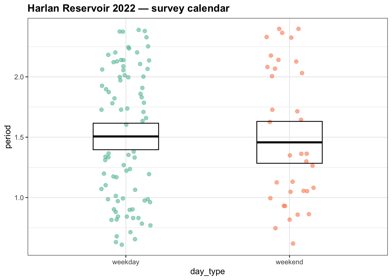
plot_design() produces a calendar visualization of which days were sampled, how they fall across strata, and where count data exist.
Code
plot_design(harlan_design, title ="Harlan Reservoir 2022 — survey calendar")
Figure 19.1: Survey calendar for the Harlan Reservoir 2022 creel survey. Each point represents a day in the sampling frame. Color distinguishes weekend and weekday strata. Filled points indicate sampled days.
The calendar makes sampling density visible. April and early May show high sampling coverage; late summer shows gaps where consecutive unsampled days cluster. These patterns matter: if the unsampled gaps are not random — if they fell on weeks with unusually poor or unusually good conditions — the stratified estimator cannot correct for them and the estimates carry unquantified bias.
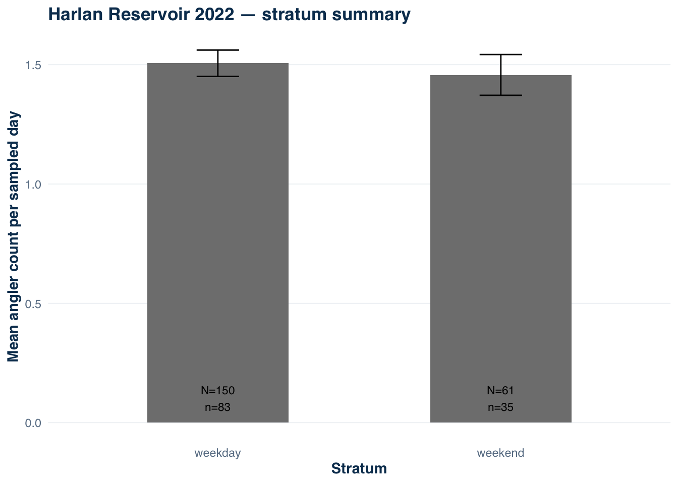
19.7 Stratum-level sampling summary
A compact view of what each stratum contributes makes it easier to catch imbalances before moving to estimation.
Warning: No shared levels found between `names(values)` of the manual scale and the
data's fill values.
No shared levels found between `names(values)` of the manual scale and the
data's fill values.
No shared levels found between `names(values)` of the manual scale and the
data's fill values.
Figure 19.2: Sample sizes and mean angler counts per stratum for the Harlan 2022 design. Error bars show one standard error of the within-stratum mean count. Numbers above bars show the population (N_h) and sample (n_h) day counts.
The mean count per sampled day is similar across strata — 31.87 for weekdays and 13.05 for weekends. Similar means across strata suggest that post-stratification by day type recovers little variance in this survey — the main value of the weekday/weekend distinction may be as a design guarantee that both day types are represented, not as a variance-reduction mechanism.
19.8 Design immutability
Each add_* function returns a new creel_design object rather than modifying its argument. This design choice prevents accidental overwriting and makes it safe to branch from any intermediate state.
Warning in svydesign.default(ids = psu_formula, strata = strata_formula, : No
weights or probabilities supplied, assuming equal probability
Code
# Build a full design branching from the same intermediate objectdesign_full <-add_interviews(design = design_counts_only,interviews = harlan_interviews_with_catch,catch ="total_harvest",effort ="hours_fished",trip_duration ="hours_fished",trip_status ="trip_status",n_anglers ="n_anglers",angler_type ="angler_type",angler_method ="angler_method",interview_type ="access")
Warning: 318 interviews have zero catch.
ℹ Zero catch may be valid (skunked) or indicate missing data.
Code
# design_counts_only is unchanged — interviews were added to design_full, not to itis.null(design_counts_only$interviews)
[1] TRUE
Immutability means the counts-only design survives the interview-addition step intact. This matters when the same count data feed multiple analysis branches — for example, effort estimation over all species (counts only) alongside harvest estimation for a target species (counts + interviews + catch). Both branches share the same intermediate object as a starting point rather than each rebuilding from scratch.
19.9 The design object as the estimation handoff
Every estimation function from Section 21.1 through Section 25.1 takes a creel_design as its first argument. The design carries the information those functions need without requiring the analyst to re-specify it at each call:
Which days were sampled and in which strata (calendar)
The realized count observations and their timing (counts)
Trip-level effort and catch totals (interviews)
Species-level catch by outcome (catch)
The underlying survey.design2 with correct strata weights
The functions that were held as eval: false placeholders in Section 10.1 — estimate_catch_rate(), validate_incomplete_trips(), and summarize_trips() — all require a creel_design object of this form. The design built in this chapter is the prerequisite for running those functions with real output.
The step-by-step build earlier in this chapter printed each intermediate state for teaching purposes. In production code, the same pipeline is written as a single pipe chain:
Warning in svydesign.default(ids = psu_formula, strata = strata_formula, : No
weights or probabilities supplied, assuming equal probability
Warning: 318 interviews have zero catch.
ℹ Zero catch may be valid (skunked) or indicate missing data.
Warning: ! Catch totals in catch data diverge from interview-level total_harvest for 329
  interviews.
ℹ This is advisory. Real creel data may differ legitimately (partial species
  recording).
The pipe chain is the production form. Each step adds one layer, and the result is a single named object that can be passed to any estimation function in the book.
19.10 What the design object stores
The creel_design object is a named list. Knowing which slot holds which information makes it possible to inspect any piece of the survey without re-running estimation.
Code
tibble(slot =c("calendar", "counts", "interviews", "catch","survey", "interview_survey","strata_cols", "date_col", "design_type"),n_rows =c(nrow(harlan_design_final$calendar),nrow(harlan_design_final$counts),nrow(harlan_design_final$interviews),nrow(harlan_design_final$catch),NA_integer_, NA_integer_, NA_integer_, NA_integer_, NA_integer_ ),contents =c("sampling schedule with sampled flag","count observations from all rounds","party-level interview records","species-level catch records","survey.design2 for count-based effort estimation","survey.design2 for interview-based estimation","stratum variable name(s)","date column name","survey design type (instantaneous, bus_route, ...)" ))
# A tibble: 9 × 3
  slot             n_rows contents
  <chr>             <int> <chr>
1 calendar            211 sampling schedule with sampled flag
2 counts              118 count observations from all rounds
3 interviews          600 party-level interview records
4 catch               987 species-level catch records
5 survey               NA survey.design2 for count-based effort estimation
6 interview_survey     NA survey.design2 for interview-based estimation
7 strata_cols          NA stratum variable name(s)
8 date_col             NA date column name
9 design_type          NA survey design type (instantaneous, bus_route, ...)
The two survey.design2 objects — design$survey and design$interview_survey — are the most important internal slots. The former carries the probability structure for estimating effort from counts; the latter carries the structure for estimating catch rates from interviews. Estimation functions pull from the appropriate slot depending on what they are estimating. Direct access to these slots is rarely needed; the estimation functions handle it internally.
19.11 When to rebuild the design
Because the design object is immutable, any change to the underlying data requires rebuilding from the affected step forward. This keeps the design aligned with the raw tables.
The most common triggers for a rebuild are:
A correction to the sampling schedule. If a day’s day_type is corrected or a day is added or removed from the sampled set, the base design must be rebuilt. A partial fix — editing the schedule but passing the old design object to estimation — will silently use the incorrect strata sizes for the N_h weights.
A catch data correction. If species totals in the catch table are revised after the design was built, add_catch() must be called again on the updated data. The species-level records inside the design object are a snapshot of the catch table at the time add_catch() was called; they do not update automatically.
An interview exclusion.Section 20.1 covers data cleaning decisions that remove or adjust specific interviews. Any such exclusion should be made on the raw interview table before the design is built, not by operating on the design object after the fact. The correct workflow is:
The harlan_design_final object built in Section 19.9 marks the end of the data preparation phase for the Harlan 2022 survey. When the next chapter’s cleaning decisions are applied, rebuild the design from the cleaned tables with the same four-step pipeline.
19.12 Takeaway
The creel_design object collects everything an estimator needs to produce a design-consistent result: the sampling frame, the strata, the realized sample counts, the party-level effort and catch, and the species-level records. Four explicit steps keep the design choices visible and verifiable.
audit_strata(), check_completeness(), and plot_design() provide immediate feedback on whether the assembled design is consistent and complete before any estimates are computed. Problems surfaced at this stage — a stratum below the minimum interview count, count dates outside the schedule, or a very high design effect — are easier to diagnose here than after estimation has already run.
The next chapter addresses data cleaning decisions that can change estimates: how to identify and handle extreme catch values, implausible trip durations, and interviews that do not pass internal consistency checks. Cleaning is done on the raw tables before building the design object.
McCormick, J. L., M. C. Quist, and D. J. Schill. 2013. Creel survey design considerations for short-duration fisheries with applications to Chinook salmon sport fisheries. North American Journal of Fisheries Management 33(3):628–641.
Pollock, K. H., C. M. Jones, and T. L. Brown. 1994. Angler survey methods and their applications in fisheries management. American Fisheries Society, Bethesda, Maryland.