creel survey, fisheries, design-based inference, R, tidycreel, Quarto
7.1 The partial-observation problem
A fishery never reveals itself all at once. On any given day, anglers are spread across shorelines and boat ramps, fishing at different times, targeting different species, departing before a technician arrives. No agency has the resources to watch every angler on every day of a season. What an agency can do is watch some anglers on some days, and then reason carefully about what those observations mean for the season as a whole.
That reasoning — from a partial view to a complete picture — is the subject of this chapter. It concerns statistical logic and the grounds for inference. On what basis can we claim that what we saw during our sampled days tells us something defensible about the days we did not sample?
The answer, when it exists, comes from the survey design. A design that selects sampling units with known probability creates a traceable connection between the observed records and the unobserved population. That connection is what transforms a collection of field notes into a scientifically defensible estimate.
The idea is easiest to see in miniature. If a 90-day season is reduced to a 30-day sample, each sampled day stands in for three similar days that were not observed. The sample only works if the 30 selected days were chosen in a way that makes that expansion legitimate.
Creel surveys are built around this principle. The methods in Pollock et al. (Pollock et al. 1994) and refined in Bernard et al. (Bernard et al. 1998) are design-based from the ground up: the expansion factors, variance estimators, and stratification schemes all depend on having defined a sampling frame, selected units from it with known probability, and recorded which units were selected and which were not. The same logic governs the tidycreel package. Understanding it at this level makes the later chapters on estimation and validation legible rather than arbitrary.
7.2 Census versus sample
Before considering how to estimate from a sample, it is worth asking what a complete census of a fishery would look like — and why it is almost never practical.
A census would require recording every angler-trip completed during the survey period: who fished, where, for how long, and what they caught. This is the standard against which samples are evaluated. Newman et al. (Newman et al. 1997) compared a stratified instantaneous-count creel survey with a complete mandatory creel census on Escanaba Lake, Wisconsin, and found that the survey-based estimates recovered the census quantities closely when the design was properly executed. That comparison is illuminating precisely because it is rare: a full census of a recreational fishery demands either a very small water body, a mandatory reporting system, or both. For most inland and coastal waters, neither condition holds.
In practice, a census would require a creel agent to be present everywhere simultaneously — at every access point, on every section of shore, for every hour of the fishing day. For a reservoir with multiple boat ramps, miles of shoreline accessible to wading anglers, and a season spanning several months, the cost is prohibitive. McCormick et al. (McCormick et al. 2013) note that complete census is “often infeasible for complex fisheries and thus is rarely used.”
The impossibility of a census creates a choice. One option is to observe whatever is convenient — survey days when the technician is available, access points that are easy to reach, anglers who happen to be leaving when the agent arrives. The other option is to select a sample deliberately, using a randomized procedure that connects the selected units back to the full population. The first option produces data. The second produces estimates.
This distinction matters because convenience data cannot support statistical inference without additional model-based assumptions. An estimate needs observations linked traceably to what was not observed. The survey design provides that link.
7.3 What makes sampling inferential
Not all partial observation supports inference. A technician who counts anglers only when convenient, interviews only approachable parties, or schedules surveys around personal preference is collecting data — but those data cannot be used to estimate population totals with statistical rigor. The estimates may be numerically plausible, but there is no formal mechanism connecting them to the population.
What transforms partial observation into a statistically defensible estimate is probability sampling: a procedure in which every unit in the sampling frame has a known, nonzero chance of being selected (Cochran 1977). Lumley (Lumley 2010) puts it plainly: “what makes a probability sample is the procedure for taking samples from a population, not just the data we happen to end up with.”
This distinction matters because the procedure — not the data — is the source of the inferential license. When a day is drawn at random from a schedule, we know its probability of selection. That probability tells us how many similar days this one day represents. When a day is selected for convenience, we have no such anchor. The field records look the same either way; the inferential status is completely different.
Nonprobability sampling — convenience samples, volunteer intercepts, opportunistic surveys — has a specific technical deficiency: there is “no scientific or theoretical basis for making meaningful statistical inference from those who were surveyed to the population they are supposed to represent” (Dillman et al. 2014). The absence of a known selection mechanism means there is no way to determine whether the observed units are representative or systematically different from the unobserved ones. Increasing the sample size from a convenience sample does not fix this problem; it just produces a larger, still-unrepresentative dataset.
The statistical properties that follow from probability sampling are powerful:
Unbiasedness: in expectation, properly weighted estimates recover the true population quantity.
Quantifiable uncertainty: variance can be estimated from the data without assuming a distributional model for the population.
Domain validity: the estimate is guaranteed to apply to the covered population frame, not to some hypothetical superpopulation.
All three properties depend on knowing, for each unit in the sample, the probability with which it was selected.
In plain language, the inclusion probability says how much of the unseen population each observed unit stands for. A unit that had a 10% chance of selection is standing in for about ten similar units that were not observed.
7.4 Notation
The design-based logic requires precise notation. Table 7.1 defines the symbols used in this chapter. Most carry forward into the estimation chapters, where they appear inside specific estimator formulas.
Table 7.1: Key notation for design-based estimation.
Symbol
Definition
N
Total number of units in the sampling frame (population size)
n
Number of units selected in the sample
\pi_i
Inclusion probability for unit i: the probability that i is selected
w_i = 1/\pi_i
Sampling weight (expansion factor) for unit i
y_i
Value of interest for unit i (e.g., angler-hours on day i)
T = \sum_{i=1}^{N} y_i
Population total
\hat{T}_{HT}
Horvitz-Thompson estimator of T
s
The realized sample (the set of selected units)
D
Number of sampling periods (fishing days) in the frame
d
Number of sampled periods
H
Stratum index (h = 1, \ldots, H)
N_h, n_h
Frame size and sample size in stratum h
\pi_h = n_h / N_h
Inclusion probability for any unit in stratum h
s_h^2
Sample variance of the y values within stratum h
\hat{V}(\hat{T})
Estimated variance of the total estimator
7.5 The sampling frame in creel surveys
The sampling frame is the explicit list — or the well-defined rule — that enumerates every unit eligible for selection. In human survey work, a frame might be a voter registration list or a telephone number registry. In creel surveys, frames are more abstract but no less important.
Pope et al. (Pope et al. in press) describe the sampling frame as “the basis of all creel surveys” and equate it with the population of inference. The frame defines what the estimate applies to. An estimate cannot legitimately describe units that were outside the frame, and a frame that omits large portions of the fishing activity produces estimates that undercount the true total even when the within-frame estimation is perfect.
In practice, creel survey frames are built from the intersection of time and space:
Temporal units: fishing days, day-type groups (weekday vs. weekend), seasonal strata, or time-of-day shifts.
Spatial units: access points, shoreline sections, water bodies, or boat launch areas.
Combined units: day-by-site or shift-by-site combinations that define the actual opportunity for a technician to be present.
The frame should include every temporal-spatial opportunity for fishing activity that the survey is intended to cover. If a reservoir is fished from five access points but only two are included in the frame, the estimate will not cover angler activity at the excluded points, regardless of how carefully the included points are sampled.
A frame is not just a list; it is a set of opportunities. Even an access point that is rarely used belongs in the frame if it is part of the fishery being described. Its low usage will reduce its contribution to the overall estimate, but excluding it removes any possibility of representing the anglers who do use it.
Consider a practical example. Calamus Reservoir in Nebraska has a primary boat ramp, a secondary ramp, and several shore-fishing areas accessible from a county road. A frame that includes only the primary ramp covers the boat fishery efficiently but misses shore anglers entirely. Whether that omission matters depends on the management question: if the goal is to estimate total harvest from all angler-types, the shore anglers must be in the frame.
The three-stage hierarchy
Most creel surveys do not select individual anglers at random from a roster. The population is not enumerable in advance — we cannot know on January 1st exactly which anglers will visit the reservoir on which days in June. Instead, selection proceeds through a hierarchy of nested units, each stage narrowing the focus until a specific field encounter becomes possible.
McCormick et al. (McCormick et al. 2013) describe the standard three-stage structure:
First stage (days): Days are randomly selected from the set of all days within the survey period or stratum. These are the primary sampling units (PSUs). The day is the unit that the analyst has the most control over and the most stake in: most of the between-sample variability in creel estimates comes from day-to-day differences in fishing activity.
Second stage (shifts): Within each selected day, a portion of the day — a shift or time window — is randomly selected for survey coverage. Not every hour of a selected day may be accessible; a shift schedule defines which time windows the technician could potentially cover, and one or more are drawn.
Third stage (count times): Within each selected shift, specific count times are drawn for instantaneous or progressive counts of anglers. Hoenig et al. (Hoenig et al. 1993) formalize the scheduling of these counts and show how the choice among simple random, systematic, and stratified count schedules affects the bias and variance of effort estimates.
This three-stage structure is a practical response to the cost of fieldwork. Surveying an entire day is expensive; surveying every count opportunity within every day is impossible. By sampling at each stage, the survey covers the full season with manageable effort while preserving the probability structure that makes expansion valid.
The hierarchy also clarifies what “replicate” means in practice. The replicate unit for estimating seasonal totals is the day, not the individual count or interview. Increasing the number of counts per day improves precision within a day but does relatively little for seasonal-level uncertainty. Increasing the number of sampled days directly reduces the primary source of variance. Newman et al. (Newman et al. 1997) demonstrated this: between-day variance dominates within-day variance in most stratified creel surveys.
Inclusion probabilities in multi-stage designs
Because selection occurs at multiple stages, the overall probability that any given angler-trip is observed is the product of selection probabilities at each stage. If a day is selected with probability \pi_d, a shift within that day is selected with probability \pi_{s|d}, and a count time within that shift is selected with probability \pi_{c|s}, then the probability that a given count observation is obtained is:
The expansion factor is the reciprocal: w_{dsc} = 1 / \pi_{dsc}. Each observed count stands in for w_{dsc} counts of the same kind that were not observed.
In most practical creel designs, the day-level probability \pi_d = n_h / N_h (within stratum h) dominates the product, because the shift and count-time selection are often implemented at high sampling fractions within the day (for example, one shift is drawn from three possible shifts, and two count times are drawn within that shift). The multi-stage nature still requires careful accounting of the joint probability; however, the simplification to a day-level expansion factor is often defensible and is the basis of most existing software implementations including tidycreel.
7.6 Inclusion probabilities and expansion factors
The inclusion probability \pi_i for a unit i is the probability that i appears in the sample under the specified design. For simple random sampling (SRS) without replacement from a frame of N units, each unit has:
\pi_i = \frac{n}{N}
For stratified designs, each unit i in stratum h has a stratum-specific probability:
\pi_i = \pi_h = \frac{n_h}{N_h}
Inclusion probabilities are the bridge between what was observed and what was not. As Breidt et al. (Breidt et al. 2009) state: “in sampling theory, the weights are the inverses of the inclusion probabilities.” A unit with \pi_i = 0.10 was selected with a 10% chance; its observation represents 10 similar units in the frame. A unit with \pi_i = 0.25 represents 4 similar units.
Two properties of inclusion probabilities are required for valid design-based inference:
Known: the probability must be calculable from the design rules. This means the schedule, the randomization procedure, and the realized sample must all be documented.
Nonzero: every unit in the frame must have a positive probability of selection. Units with zero inclusion probability are effectively excluded from the frame.
A unit with an unknown inclusion probability cannot be weighted correctly. If some days or sites were surveyed outside the formal randomization procedure — opportunistically, or as fill-ins — those days carry unknown inclusion probabilities. Including them at the nominal schedule weight is incorrect; excluding them may introduce bias. Neither option is satisfactory, which is why deviation from the scheduled design must be documented and handled explicitly.
7.7 The Horvitz-Thompson estimator
The central result in design-based survey sampling is the Horvitz-Thompson (HT) estimator, introduced by Horvitz and Thompson (Horvitz and Thompson 1952) and foundational to creel estimation since Robson (Robson 1961).
For a population of N units, let y_i denote the value of interest for unit i. The population total is T = \sum_{i=1}^{N} y_i. We observe a sample s of n units. The Horvitz-Thompson estimator of T is:
where w_i = 1/\pi_i is the sampling weight for unit i.
The estimator is unbiased: E(\hat{T}_{HT}) = T. The proof is brief. By the properties of expectation over all possible samples the design could generate:
Each unit i contributes y_i / \pi_i to the sum when it appears in s, which happens with probability \pi_i, so its expected contribution is exactly y_i. Summing over all units recovers T.
The intuition is equally direct. If a day is selected with probability \pi_i = d/D — that is, d days are drawn at random from a frame of D total days — then the expansion factor is D/d. The observed count on that day, multiplied by D/d, gives the contribution to the seasonal total. Summing across all sampled days yields the estimate. The structure total = mean-per-unit × number-of-units is the HT estimator in applied form; it is not a heuristic.
Bernard et al. (Bernard et al. 1998) give this formulation explicitly for harvest estimation in a two-stage roving-access design. Their equation for seasonal harvest \hat{H} within a stratum is:
\hat{H} = \frac{D}{d} \sum_{i=1}^{d} \hat{H}_i
where D is the number of fishing days in the frame, d is the number sampled, and \hat{H}_i = \hat{E}_i \times \widehat{HPUE}_i is harvest estimated within sampling period i as the product of estimated fishing effort and estimated mean harvest rate. When periods are selected by SRS, \pi_i = d/D for all i, and the Bernard formula is exactly the HT estimator.
A worked numeric example
To make the HT estimator concrete, apply it to the Harlan Reservoir dataset. The schedule table records both the total number of eligible days per stratum (N_h) and which days were sampled (n_h). The counts table records how many anglers were observed on each sampled day.
Code
harlan_schedule <-readRDS(here("data/harlan_schedule.rds"))harlan_counts <-readRDS(here("data/harlan_counts.rds"))# Bank anglers are counted directly; boats are counted and expanded by the# mean anglers per boat party measured in the interviews.harlan_counts <-derive_angler_count( harlan_counts,bank = bank_anglers,boat_count = angler_boats,party_size =mean_party_size(harlan_interviews, n_anglers, angler_type = angler_type))# Stratum frame sizes and sample sizes from the schedulestrata <- harlan_schedule |>group_by(day_type) |>summarise(N =n(), n_sampled =sum(sampled), .groups ="drop") |>filter(!is.na(day_type))strata
# A tibble: 2 × 3
  day_type     N n_sampled
  <chr>    <int>     <int>
1 weekday    150        82
2 weekend     61        34
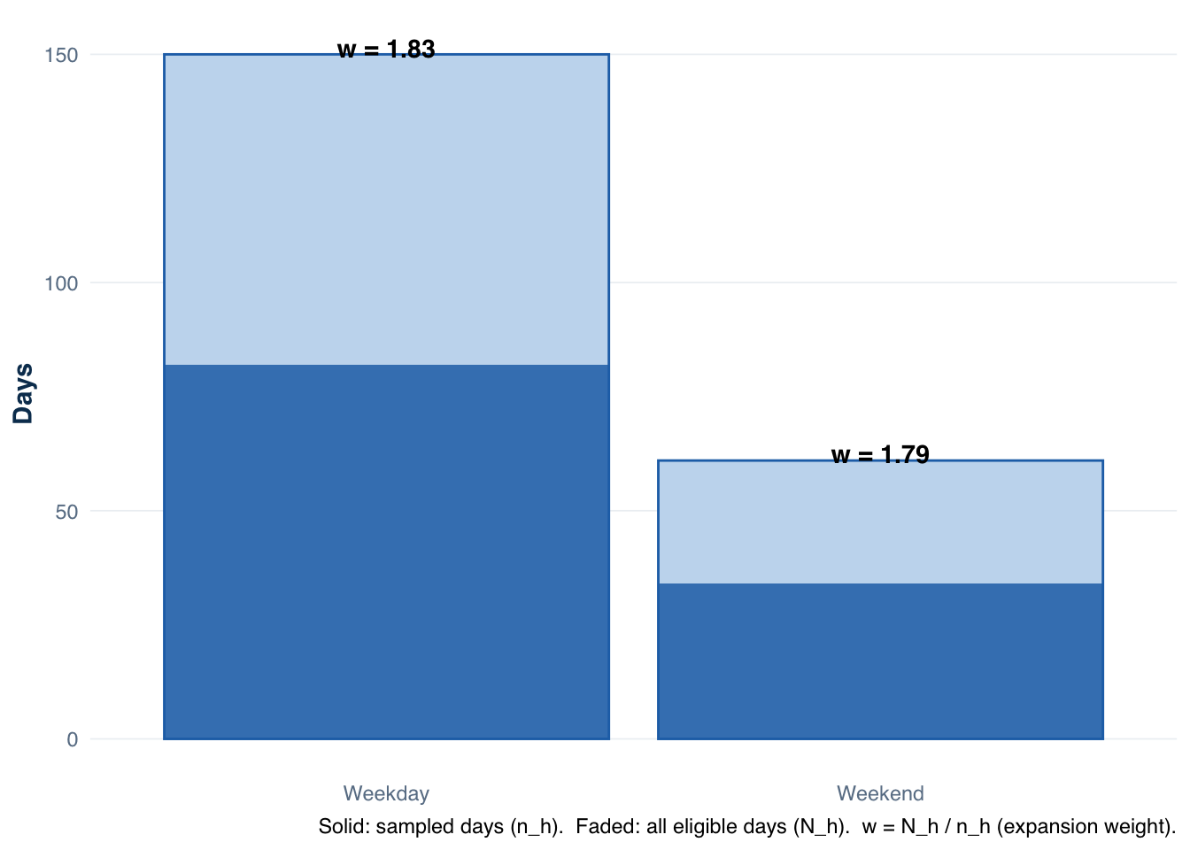
Figure 7.1 translates these frame and sample sizes into the inclusion probabilities and expansion weights that drive the HT estimator. Each sampled day stands in for N_h / n_h similar days in the stratum.
Code
strata |>mutate(label =c(weekday ="Weekday", weekend ="Weekend")[day_type],w =round(N / n_sampled, 2) ) |>ggplot(aes(x = label)) +geom_col(aes(y = N), fill ="#c6dbef", colour ="#2171b5", linewidth =0.5) +geom_col(aes(y = n_sampled), fill ="#2171b5", alpha =0.85) +geom_text(aes(y = N +1.5, label =paste0("w = ", w)),size =3.8, fontface ="bold" ) +labs(x =NULL,y ="Days",caption ="Solid: sampled days (n_h). Faded: all eligible days (N_h). w = N_h / n_h (expansion weight)." ) +theme_creel()
Figure 7.1: Sampling fractions and expansion weights by stratum at Harlan Reservoir. Light bars show total eligible days per stratum (N_h); solid bars show sampled days (n_h). The expansion weight w = N_h / n_h, printed above each bar, is the factor applied to each sampled day in the HT estimator. Both strata were sampled at similar rates (~55%), so their weights are comparable.
The daily y_i values — the quantity we want to total over all days — are the sums of anglers counted per sampled day. Here we use the sum of boat and bank anglers across all count periods within each day as a measure of daily fishing activity.
The seasonal total is the sum of two stratum-level HT estimates, each weighted by its expansion factor N_h / n_h. The weekday expansion factor (150/82 \approx 1.83) and weekend expansion factor (61/34 \approx 1.79) are similar here — Harlan’s design sampled both strata at roughly comparable rates (~55%). The confidence interval width reflects between-day variability in counts (the s_h^2 terms) and the remaining unsampled fraction in each stratum (the finite-population correction).
Note that y_i here is a raw count index, not angler-hours. The estimate_effort() function in tidycreel extends this framework to convert counts to hours using shift duration and mean trip duration from interviews, as covered in Chapter 4.
The seasonal total is the sum of stratum-level HT estimates, each stratum contributing according to its own expansion factor. Strata sampled at a higher rate (more n_h relative to N_h) receive a smaller expansion factor because each sampled day represents fewer unsampled days. Strata sampled less intensively receive larger weights.
Unequal weights and what they mean
The different stratum expansion factors in the example above are a direct consequence of different sampling intensities, not an error or approximation. When the design allocates sampling effort disproportionately across strata — sampling weekends at a higher rate than weekdays — the resulting weights are unequal by design. Applying a single, pooled expansion factor to all days (for example, 60/18 = 3.33) would overexpand weekday records and underexpand weekend records, biasing both stratum totals and the seasonal estimate.
This is why the expansion weight must always come from the actual selection probability, not from a convenient approximation. The rule is simple: w_i = 1/\pi_i, where \pi_i is the documented inclusion probability for unit i. Departing from this rule without explicit justification introduces bias that may not be apparent from the data alone.
7.8 Design-based versus model-based inference
There are two fundamentally different philosophical stances toward statistical estimation from a sample. Understanding the difference matters because creel survey analysis sits squarely within one of them — and mixing them up is a common source of error.
Design-based inference treats the population values as fixed, deterministic constants. The fishing pressure on a specific Tuesday in July is a real number — it is not a random variable. The only randomness in the system comes from the act of sampling: whether that Tuesday happened to be selected, which count times were drawn, which anglers were intercepted. Uncertainty in the estimate reflects the variability across all the samples the design could have generated, not a distributional assumption about angler behavior.
As Ida et al. (Ida et al. 2014) state it: “the variable interest values for each population unit are considered to be deterministic and the only variable present is that of the construction of the sample. The statistical inference then only describes the randomness created by the sampling design.”
Model-based inference treats the population values as realizations of a random process. Under this view, the 47 angler-hours observed on a Tuesday is a draw from some probability distribution that governs Tuesday fishing effort. Uncertainty comes from the assumed model, not from the sampling procedure. With strong model assumptions, you can estimate population quantities even from convenience samples — because the model provides the inferential mechanism that the design would otherwise supply.
The practical differences are substantial:
Table 7.2: Comparison of design-based and model-based inference frameworks.
Property
Design-based
Model-based
Source of randomness
Sampling procedure
Assumed data-generating process
Validity requires
Known inclusion probabilities
Correct model specification
Robustness
Valid under any population structure
Valid only if model is correct
Variance estimation
From design alone
From model residuals
Convenience samples
Cannot rescue
May partially rescue
Design-based methods are robust in an important sense: the HT estimate is valid regardless of the true distribution of fishing effort across days. Whether effort follows a normal distribution, a log-normal distribution, or no recognizable distribution at all, the HT estimator is unbiased as long as the design was faithfully executed. No distributional assumption is needed because the sampling procedure provides the probabilistic scaffold.
Model-based methods can be valuable when direct estimation is not possible — for estimating quantities in subgroups too small to support the HT estimator, for combining creel data with auxiliary information, or for predicting effort at unsampled access points. But validity depends entirely on how well the model describes the data-generating process. A model that assumes fishing effort is proportional to air temperature will give biased estimates in fisheries where temperature and effort are uncorrelated.
Lumley (Lumley 2010) makes the practical implication explicit for regression applied to survey data: “all the statistical inference in this chapter is still design-based and its validity makes no assumptions about the truth of the model or the distribution of any variable.” Even when a regression model is incorporated into the analysis — for ratio estimation or domain estimation — the design-based framework requires that the variance be computed from the design structure, not from model residuals alone.
This book uses design-based methods throughout, following the framework established by Pollock et al. (Pollock et al. 1994) and Bernard et al. (Bernard et al. 1998) for creel survey estimation. The estimators that tidycreel implements are grounded in the design.
7.9 Variance from the design
An estimate without uncertainty is not complete. A seasonal total of 1,400 angler-hours carries very different implications if the 95% confidence interval spans 800 to 2,000 angler-hours versus 1,300 to 1,500 angler-hours. The width of that interval depends on how the sample was designed.
Wolter (Wolter 2007) states this plainly: “a common error of the survey practitioner or the beginning student is the belief that simple random sampling formulae may be used to estimate variances, regardless of the design or estimator actually employed. This belief is false. An estimator of variance must take account of both the estimator and the sampling design.”
For the HT estimator under simple random sampling without replacement from a frame of N units, the exact variance is:
where S^2 = \frac{1}{N-1}\sum_{i=1}^{N}(y_i - \bar{Y})^2 is the population variance of the unit values. The term (1 - n/N) is the finite population correction (fpc): it shrinks toward zero as the sampling fraction n/N approaches one, reflecting the fact that a census (n = N) has no sampling uncertainty. For typical creel survey sampling fractions (often 10–30% of days), the fpc is non-negligible and should be included.
In practice, S^2 is unknown and is estimated from the sample:
The stratum-level terms reveal which strata contribute most to overall uncertainty. A stratum with high day-to-day variability in fishing effort (large s_h^2) or low sampling intensity (small n_h / N_h) inflates the variance estimate. This drives the allocation logic in Chapter 7: to minimize total variance, allocate more sampling effort to strata where effort is more variable.
Variance components in multi-stage designs
In the three-stage creel design, variance decomposes into components corresponding to each stage. Bernard et al. (Bernard et al. 1998) give the two-stage variance for seasonal harvest as:
The first term is the between-period variance: how much the per-day harvest estimates \hat{H}_i vary across sampled days. The second term is the within-period variance: how much uncertainty remains in \hat{H}_i because not every angler on a sampled day was interviewed.
For a strategically designed survey, between-period variance almost always dominates. If anglers fish more on some days than others — which is universally true — then sampling more days is the primary lever for improving seasonal precision. Increasing the count frequency within a day improves within-day effort estimates but does relatively little for the seasonal total if day-to-day variability is large.
The dominance of between-period variance — which is typical of creel surveys — has an immediate practical implication: allocating survey effort toward more days rather than more intensive coverage of fewer days usually improves precision more efficiently. This is not a rule of thumb; it follows directly from the variance decomposition.
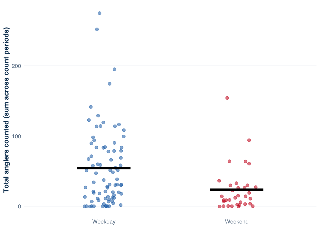
Figure 7.2 shows the day-to-day variability in total observed anglers across sampled days at Harlan, split by stratum. The spread within each stratum is the s_h^2 term that drives the variance formula. Days with unusually high or low counts are the observations that dominate sampling uncertainty — no amount of additional within-day counting can reduce the uncertainty contributed by missing those days from the sample.
Figure 7.2: Day-to-day variability in total observed anglers at Harlan Reservoir by day type. Each point is one sampled day. The spread within each stratum (the between-day standard deviation) is the primary driver of seasonal estimate uncertainty. More sampled days reduces this uncertainty directly; more counts per day does not.
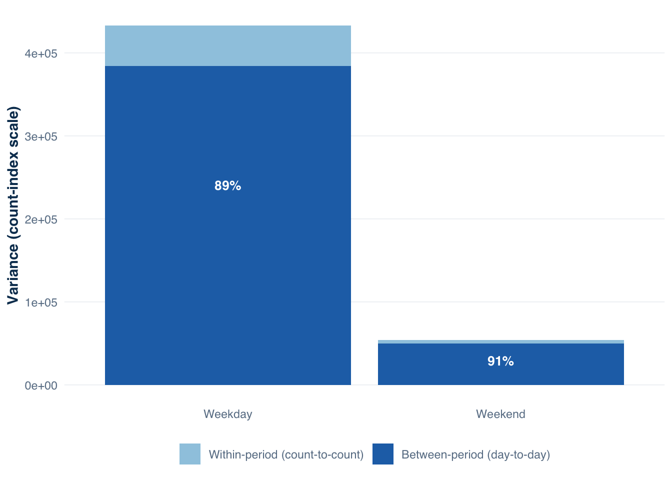
Figure 7.3 quantifies how variance decomposes into between-period and within-period components for both strata. The dominance of between-period variance confirms that the priority for improving seasonal precision is more sampled days, not more counts per day already in the sample.
Warning in data.frame(label = c(weekday = "Weekday", weekend = "Weekend")[st],
: row names were found from a short variable and have been discarded
Warning in data.frame(label = c(weekday = "Weekday", weekend = "Weekend")[st],
: row names were found from a short variable and have been discarded
Figure 7.3: Variance decomposition by stratum at Harlan Reservoir. Between-period variance (day-to-day variability in angler activity) accounts for nearly all total variance in both the weekday and weekend strata. Within-period variance (variability in counts across time periods within a sampled day) is negligible. Adding sampled days directly reduces the dominant component; adding count periods per day addresses only the minor component.
The design effect
The design effect (deff) is a measure of how much the chosen design inflates or deflates variance relative to what simple random sampling of the same size would produce:
A design effect of 2.0 means the design is twice as variable as SRS with the same n; equivalently, the effective sample size is n / \text{deff} = n/2. Design effects greater than one arise from clustering (days within strata tend to be more similar than randomly selected days across the full season) and from unequal weighting (strata sampled at very different rates). Design effects less than one can arise from stratification when strata are homogeneous within but different between, because the design prevents overrepresentation of any one stratum.
McCormick et al. (McCormick et al. 2013) note that the design effect in creel surveys “has not been extensively evaluated in short-duration fisheries,” partly because the comparison baseline (SRS of individual trips) is operationally impossible. Nonetheless, understanding deff helps analysts evaluate whether their stratification and allocation choices are paying off in efficiency terms.
7.10 What the design authorizes
Design-based inference is specific about what an estimate can and cannot claim.
What it can claim: the estimate applies to the population of units in the sampling frame, within the time period and spatial domain covered by the survey. A seasonal total derived from a stratified random sample of fishing days at a reservoir during June–August is a defensible estimate of angling activity at that reservoir during that period, under the assumption that the frame covered all relevant fishing opportunities and that the design was faithfully executed.
What it cannot claim: the estimate does not automatically generalize to other time periods, other water bodies, or units outside the frame. A survey that covered only the boat ramp access points cannot estimate activity at shore-fishing locations. A survey conducted from June through August cannot estimate September harvest. These extrapolations require either additional design coverage or explicit model-based assumptions — and those assumptions should be stated and scrutinized.
This domain-specificity is not a peculiarity of creel surveys. It is a property of all design-based estimates. The scope of the claim matches the scope of the design. Extending the claim beyond the design requires a deliberate justification.
The authorization chain
The design-based framework can be stated as a chain of authorizations, each step depending on the previous:
Define the target population: all angler-trips completed on the study water during the survey period.
Build the sampling frame: enumerate or define all temporal-spatial units that provide opportunities to observe angler activity.
Select sampling units with known probability: randomly assign days, shifts, and count times to the sample using a documented procedure.
Execute the design: conduct counts and interviews according to protocol; document deviations.
Weight by inclusion probability: attach expansion factors derived from the selection probabilities, not from post-hoc judgment.
Estimate population quantities: apply the appropriate estimator (HT for totals; ratio estimators for catch rates).
Quantify uncertainty: compute variance from the design equations, not from generic formulas.
State the inference: describe what population, time period, and domain the estimate covers.
Each link depends on the previous one. Skipping step 3 — using a convenience sample — breaks the chain at the point where statistical inference would otherwise be authorized. Applying wrong weights at step 5 produces a biased total even if every other step was correctly executed. Reporting a point estimate without uncertainty at step 7 obscures the precision of the result.
Pope et al. (Pope et al. in press) are direct: “all estimates must be accompanied by some measure of variation (e.g., variance, standard error, and 95% confidence interval).” This is not stylistic preference. It is a statement about what constitutes a complete scientific result.
7.11 Failure modes
The design-based logic breaks down in predictable ways. Recognizing these failure modes is as important as understanding the ideal case.
Frame undercoverage: the sampling frame omits a portion of the fishery. If an access point was excluded because it is difficult to reach, all angling activity at that point is invisible to the estimate. The bias is systematic and cannot be corrected by increasing sample size within the covered frame.
Unknown inclusion probabilities: a unit was surveyed outside the formal randomization — as a fill-in, or because conditions were favorable. That unit carries an unknown probability of selection and cannot be weighted correctly. Including it at the nominal schedule weight is wrong; excluding it may introduce bias.
Protocol drift: the field protocol specifies randomly scheduled counts, but technicians in practice survey when anglers are most active. The nominal inclusion probabilities remain correct on paper, but the realized selection is no longer random. Estimates may be biased toward high-use periods.
Domain extrapolation: an estimate derived from one stratum or access point is reported as if it applies to the whole fishery. The design did not cover the whole fishery, so the estimate cannot describe it.
Data cleaning that changes selection: a record is excluded from analysis because of a data entry error, but the excluded day was part of the random sample. Removing it without adjustment changes the effective inclusion probability and introduces bias. Bernard et al. (Bernard et al. 1998) develop methods for handling missing data within sampled periods precisely because this failure mode is operationally common.
Applying SRS variance formulas to clustered data: Wolter (Wolter 2007) identifies this as “a common error.” Days within a stratified creel design are not independent draws from the full population; they are nested within strata and selected in a structured way. The SRS variance formula underestimates true variance when clustering is present and overestimates it when stratification reduces variability. Neither error direction is predictable in advance.
7.12 Connecting to tidycreel
The tidycreel package encodes the design-based logic at each stage of the workflow. The connection between concepts and functions is direct.
Frame and schedule — generate_schedule() builds the stratified random calendar that constitutes the operational sampling frame. The arguments define the strata (day types, seasons), the total frame size (N_h), and the number of units to sample in each stratum (n_h). The output records which units are sampled and, implicitly, the inclusion probability \pi_h = n_h / N_h for each stratum.
Code
# Build a stratified random schedule for a 90-day seasonschedule <-generate_schedule(start_date ="2024-04-01",end_date ="2024-06-30",n_periods =2L,n_days =c(weekday =15, weekend =12),seed =42)# Inclusion probabilities are implicit in the strata allocation:# weekday: 15/65 ≈ 0.23 (65 weekdays in Apr–Jun)# weekend: 12/26 ≈ 0.46 (26 weekend days in Apr–Jun)head(schedule)
April 2024
Sun
Mon
Tue
Wed
Thu
Fri
Sat
WEEKD
02
03
04
05
06
WEEKE
08
WEEKD
10
11
12
13
14
15
16
17
18
19
20
21
22
23
24
25
26
27
28
29
30
The schedule object is the frame made operational. Every day in the season is represented; sampled days are flagged. The ratio of sampled to total days within each stratum gives \pi_h, which downstream estimation functions use to compute expansion weights automatically.
Design object — creel_design() attaches counts, interviews, and catch records to the schedule, constructing a structured representation that preserves the link between observations and the frame. The design object is what makes estimation functions aware of the stratification and weighting structure.
Estimation — estimate_effort(), estimate_total_catch(), and related functions apply the weighted HT expansion equations internally. They read the design structure rather than requiring the analyst to supply expansion weights manually, reducing the opportunity for weighting errors — which, as shown above, are a common source of bias.
The package can represent the design, but it cannot rescue a missing frame or recover a probability structure that was never created in the field. If the schedule was not randomized, generate_schedule() can generate a random schedule on request — but that schedule applies to the analysis only if the field work followed it. The design-based guarantee comes from what happened in the field, not from the software.
7.13 Summary
Design-based creel estimation rests on four pillars:
A frame: an explicit or well-defined enumeration of every unit eligible for selection, covering the intended population.
Known inclusion probabilities: every sampled unit was selected through a documented random procedure with a calculable probability.
Correct weighting: expansion factors are derived from the inclusion probabilities, not from convenience or convention.
Design-appropriate variance: uncertainty is quantified using formulas that match the stratification, clustering, and multi-stage structure of the design.
When all four are in place, the estimate carries a formal guarantee: it is unbiased in expectation, its uncertainty is quantifiable without distributional assumptions, and its scope of inference is precisely defined by the frame. That guarantee is what distinguishes a creel survey estimate from an informed guess — however numerically similar the two might look.
The chapters that follow build on this foundation. Chapter 4 applies the framework to access-point designs; Chapter 5 to roving designs. The estimation chapters in the second half of the book implement the specific estimators for effort, catch, harvest, release, and CPUE. In each case, the design-based logic described here is what makes those estimators defensible rather than merely convenient.
Bernard, D. R., A. E. Bingham, and M. Alexandersdottir. 1998. Robust harvest estimates from on-site roving–access creel surveys. Transactions of the American Fisheries Society 127(3):481–495.
Breidt, F. J., H. Lai, J. D. Opsomer, and D. A. Voorhees. 2009. Improved estimation methods for the access point angler intercept survey component of the marine recreational fishery statistics survey. NOAA Technical Memorandum NMFS-F/SPO-102.
Cochran, W. G. 1977. Sampling techniques, 3rd edition. John Wiley & Sons, New York.
Dillman, D. A., J. D. Smyth, and L. M. Christian. 2014. Internet, phone, mail, and mixed-mode surveys: The tailored design method, 4th edition. John Wiley & Sons, Hoboken, New Jersey.
Hoenig, J. M., D. S. Robson, C. M. Jones, and K. H. Pollock. 1993. Scheduling counts in the instantaneous and progressive count methods for estimating sportfishing effort. North American Journal of Fisheries Management 13(4):723–736.
Horvitz, D. G., and D. J. Thompson. 1952. A generalization of sampling without replacement from a finite universe. Journal of the American Statistical Association 47(260):663–685.
Ida, B., L.-P. Rivest, and G. Daigle. 2014. Using balanced sampling in creel surveys. Environmetrics 25(2):95–110.
Lumley, T. 2010. Complex surveys: A guide to analysis using R. John Wiley & Sons, Hoboken, New Jersey.
McCormick, J. L., M. C. Quist, and D. J. Schill. 2013. Creel survey design considerations for short-duration fisheries with applications to Chinook salmon sport fisheries. North American Journal of Fisheries Management 33(3):628–641.
Newman, S. P., P. W. Rasmussen, and L. M. Andrews. 1997. Comparison of a stratified, instantaneous count creel survey with a complete mandatory creel census on Escanaba Lake, Wisconsin. North American Journal of Fisheries Management 17:321–330.
Pollock, K. H., C. M. Jones, and T. L. Brown. 1994. Angler survey methods and their applications in fisheries management. American Fisheries Society, Bethesda, Maryland.
Pope, K. L., C. J. Chizinski, A. J. Lynch, and J. R. Post. in pressin press. Creel surveys.
Robson, D. S. 1961. On the statistical theory of a roving creel census of fishermen. Biometrics 17(3):415–437.
Wolter, K. M. 2007. Introduction to variance estimation, 2nd edition. Springer, New York.