11Aerial, Camera-Assisted, and Remote Count Designs
Author
Christopher Chizinski
Keywords
creel survey, fisheries, design-based inference, R, tidycreel, Quarto
11.1 Why remote counts?
Standard creel survey designs — access-point (Section 9.1) and roving (Section 10.1) — assume a field crew can stand at an access point or travel a route and count anglers directly. That assumption fails when the waterbody is too large for crew coverage, when weather prevents reliable manual counts, when budget limits staffing to only a few days per week, or when the survey requires higher temporal resolution than a crew can provide.
Remote and technology-assisted count methods solve the coverage problem by replacing or supplementing the human observer with a sensor — a camera at a boat ramp, an aircraft flying a systematic route, a vehicle counter at a road crossing. Coverage goes up, field labor goes down, and the record becomes persistent: a camera image can be reviewed; a flight log can be audited.
The estimation logic does not change. Effort is still the product of a count of anglers and the hours those anglers were available to fish. What changes is how the count is collected and how timing uncertainty is handled. An aerial flight covers the entire waterbody in thirty minutes but captures only a snapshot at the flight time. A boat-ramp camera records every ingress event but produces a vehicle count, not a direct angler-hour measurement. Both require a link between the count and total effort — through a model, through a calibration ratio, or through mean trip length from interviews.
tidycreel provides dedicated design types and estimators for each major remote-count approach: design_type = "aerial" with estimate_effort_aerial_glmm() for time-of-day-adjusted aerial surveys, and design_type = "camera" with est_effort_camera() for ingress/egress counter designs. The same creel_design() → add_counts() → add_interviews() → estimate pipeline applies to both, with a few additional required arguments that capture the characteristics of the observation system.
The common thread is simple: the remote sensor changes how the count is observed, but not what the analyst needs for inference. The target is still angler-hours, so each design has to translate the sensor output back into that unit.
11.2 Aerial surveys
The observation problem
An aerial survey produces one count per flight, and the count reflects the number of anglers visible at a single moment in time. Angler density on a lake changes continuously across the fishing day: low at first light, building through midmorning as anglers arrive, peaking around midday or early afternoon, then declining as anglers leave and daylight wanes. A single flight at 10:00 captures a different density than a flight at 14:00 on the same day.
The naive expansion — count × hours_open — assumes the observed density is representative of the full day, which it is only if the flight happens exactly at the time when mean daily density occurs. If flights are consistently timed early or late relative to peak use, the effort estimate is biased in a predictable direction.
The standard fix is a time-of-day model that predicts how angler density varies across the fishing day. Multiple flights on the same days, spaced at different times, provide the data to fit that model. The fitted curve is then integrated across the full open-water period to recover total daily effort. estimate_effort_aerial_glmm() fits this model as a generalized linear mixed model (GLMM) with a quadratic time-of-day effect and a day-level random intercept:
where t is flight time, u_d \sim N(0, \sigma^2) is a day-level random effect that absorbs day-to-day variation in total use, and the exponential link keeps predictions non-negative. Integrating the fitted curve over the h_{\text{open}} open hours of the fishing day recovers a day-specific total angler-hours estimate, which is then expanded to the full season using the stratified ratio estimator.
Data structure
An aerial survey dataset contains one row per flight observation — not one row per day. Multiple flights on the same day appear as separate rows, linked by date and distinguished by time_of_flight. The tidycreel bundled dataset example_aerial_glmm_counts illustrates this structure:
Four flights per day at hours 7, 10, 13, and 16. The counts rise from early morning to a midday peak, then fall — exactly the pattern the GLMM is designed to capture. With four time points per day, the quadratic curve is well constrained.
Building the aerial design
An aerial design requires four additions to the standard creel_design() call:
design_type = "aerial" — routes count data to the GLMM estimator
h_open — total fishing hours per day (daylight hours accessible to anglers)
Raw, unaggregated counts passed to add_counts() without count_time_col, so time_of_flight is preserved in design$counts for the model
visibility_correction and angler_ratio — the two corrections that turn a raw observer count into an angler count
An aerial count is what an observer saw from a moving aircraft, and it is wrong in two directions at once. Some anglers were missed, which biases the count down; some of the people who were seen were not fishing, which biases it up. Smucker et al. (2010) correct both, and tidycreel requires you to state both. There is deliberately no default. Supplying nothing is not the same claim as declaring that no correction applies, and only one of those should be silent — so an aerial design that names neither correction raises an error rather than quietly assuming perfect detection and an all-angler shoreline.
visibility_correction is a detection probability: the proportion of present anglers the observer saw. Field studies do not report it that way. They report a ground-truthing ratio r = \text{ground} / \text{aerial}, which exceeds 1 exactly when the correction matters, so you pass its reciprocal v = 1/r. For the shore mode Smucker et al. (2010) report r = 4.421 (SE 0.864) — aerial counts caught under a quarter of the shore anglers actually present — giving v = 0.226. The standard error transforms with the point estimate: for a reciprocal, \mathrm{SE}(1/r) = \mathrm{SE}(r)/r^2 = 0.0442.
angler_ratio is the angler-to-people ratio, and it pushes the other way: only about 40% of the people visible along the bank were fishing. The two corrections therefore partly cancel, which is precisely why applying one alone is not the conservative choice — it biases the estimate in the direction of whichever correction you kept.
Both arguments accept standard errors, and you should supply them whenever the source reports them. A correction estimated from paired counts is not a known constant, and an effort estimate that treats it as one reports a standard error that is too small. If a correction genuinely does not apply, say so explicitly with visibility_correction = "none"; the point estimate then uses 1 and the reported standard error is NA — never 0, which would be indistinguishable from having propagated the uncertainty and found none.
Code
aerial_calendar <-tibble(date =seq(min(example_aerial_glmm_counts$date),max(example_aerial_glmm_counts$date), by ="day"),day_type =if_else(wday(date) %in%c(1L, 7L), "weekend", "weekday"))design_aerial <-creel_design(calendar = aerial_calendar,date ="date",strata ="day_type",design_type ="aerial",h_open =14,# Shore mode, Smucker et al. (2010) table 3: the ground-truthing ratio is# 4.421 (SE 0.864). tidycreel wants the detection probability v = 1/r, and# the SE of a reciprocal is se(r)/r^2 = 0.864 / 4.421^2.visibility_correction =0.2262,visibility_se =0.0442,# Their table 2, May: the angler-to-people ratio is 0.402 (SE 0.0360).angler_ratio =0.402,angler_ratio_se =0.0360) |>add_counts(example_aerial_glmm_counts, count_col = n_anglers) |>add_interviews(interviews = example_aerial_interviews,catch ="walleye_catch",harvest ="walleye_kept",effort ="hours_fished",trip_status ="trip_status",trip_duration ="hours_fished" )
Warning in add_counts(creel_design(calendar = aerial_calendar, date = "date", : `counts` has 36 repeated sampling units, with no count time to tell them apart.
ℹ The repeated rows are keyed on date and day_type.
ℹ Estimators that sum these rows refuse them; supply `count_time_col` if they
  are repeat counts, or `unit_cols` if they are distinct units.
Warning in svydesign.default(ids = psu_formula, strata = strata_formula, : No
weights or probabilities supplied, assuming equal probability
Warning: ! No `n_anglers` provided — assuming 1 angler per interview.
ℹ Pass `n_anglers = <column>` to use actual party sizes for angler-hour
  normalization.
ℹ If the interviews really are one angler each, pass `n_anglers = 1` to state
  that and silence this warning.
Warning: 15 interviews have zero catch.
ℹ Zero catch may be valid (skunked) or indicate missing data.
The contrast with a standard instantaneous design is in design_type and h_open. Everything else — add_interviews(), estimation calls — follows the same pattern. The GLMM handles the time-of-day adjustment internally; the analyst provides the data and the open-water window.
Time-of-day pattern
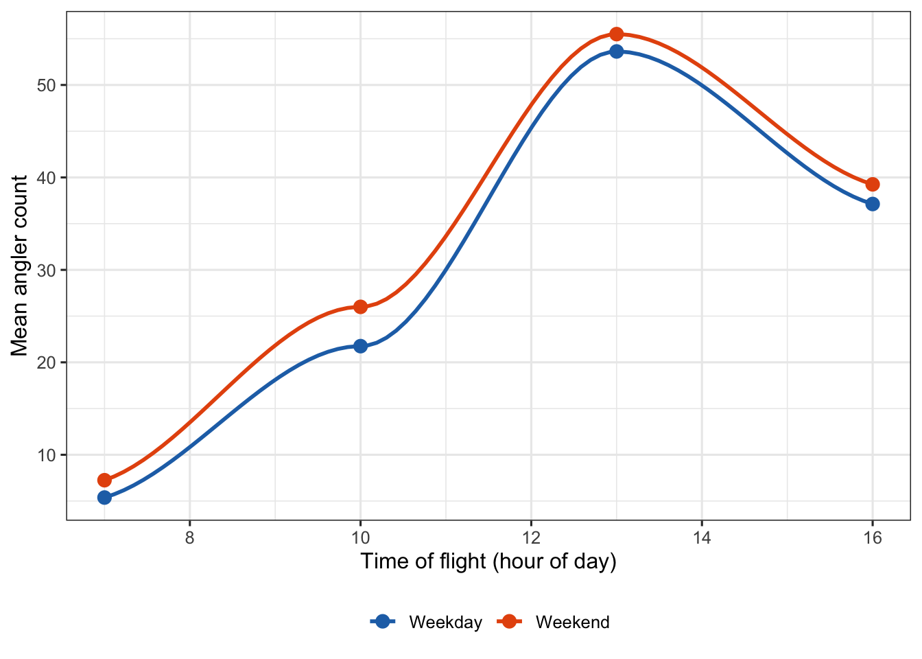
Before estimating effort, it is worth visualizing what the GLMM is fitting. Figure 11.1 shows mean count by flight time across both day types, with the quadratic pattern that drives the model.
Warning in simpleLoess(y, x, w, span, degree = degree, parametric = parametric,
: reciprocal condition number 0
Warning in simpleLoess(y, x, w, span, degree = degree, parametric = parametric,
: There are other near singularities as well. 36.542
Figure 11.1: Mean aerial count by time of flight and day type. Points show stratum means across sampled days; the curve is a loess smoother that approximates the quadratic GLMM fit. Counts peak in early afternoon and are consistently higher on weekends, reflecting higher recreational use.
The inverted-U shape confirms that a single flight at 07:00 would underestimate total daily effort, while a flight at 13:00 would overestimate it. The GLMM integrates the full curve rather than multiplying one snapshot count by hours_open.
That is the reason the model is doing real work here. It is not just smoothing noise; it is replacing a one-time observation with a full-day representation of use.
Estimating effort
estimate_effort_aerial_glmm() fits the negative-binomial GLMM, integrates the fitted curve across h_open hours, and expands to the full season using the stratified frame. The result is a total angler-hours estimate for the survey period with a delta-method standard error.
ℹ Integration window start derived from data: 6.5 h (earliest flight - 0.5 h).
  Specify `open_start` in `creel_design()` for a fixed fishery opening time.
Code
effort_aerial
── Creel Survey Estimates ──────────────────────────────────────────────────────
Method: aerial_glmm_total
Variance: delta
Confidence level: 95%
model: 58.62 (included in se)
visibility: 131.5 (included in se)
angler_ratio: 60.25 (included in se)

# A tibble: 1 × 7
  estimate    se se_between se_within ci_lower ci_upper     n
     <dbl> <dbl>      <dbl>     <dbl>    <dbl>    <dbl> <int>
1     673.  156.       156.        NA     367.     979.    48
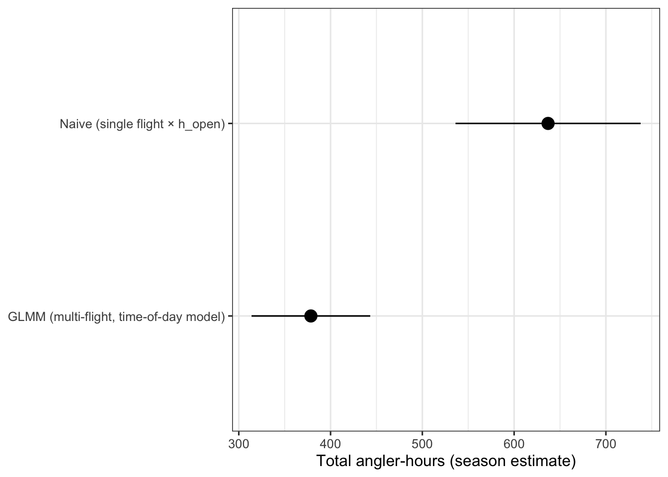
The GLMM estimates 673 total angler-hours (95% CI: 367–979). The total and its standard error reflect two sources of variance: between-day variation in total use (absorbed by the GLMM day-level random effect) and between-stratum variation in sampling intensity (handled by the stratified expansion). The ratio of se_between to total se indicates how much of the uncertainty comes from which-days-were-sampled versus which-time-flights-were- conducted.
The GLMM requires lme4. If the package is not installed, tidycreel will prompt installation before the call proceeds.
Naive estimate vs GLMM
To see what the time-of-day correction buys, it helps to compare the GLMM result against the naive single-flight expansion. example_aerial_counts contains one count per day — a midmorning flight — that can be treated as a standard instantaneous-count design using estimate_effort():
Code
# Standard instantaneous design with one flight per day# h_open goes into creel_design(), not estimate_effort()design_naive <-creel_design(calendar = aerial_calendar,date ="date",strata ="day_type",h_open =14) |>add_counts(example_aerial_counts) |>add_interviews(interviews = example_aerial_interviews,catch ="walleye_catch",harvest ="walleye_kept",effort ="hours_fished",trip_status ="trip_status",trip_duration ="hours_fished" )effort_naive <-estimate_effort(design_naive)effort_naive$estimates
# A tibble: 1 × 7
  estimate    se se_between se_within ci_lower ci_upper     n
     <dbl> <dbl>      <dbl>     <dbl>    <dbl>    <dbl> <int>
1      637  47.0       47.0         0     536.     738.    16
Figure 11.2: Aerial effort estimates from a naive single-flight expansion versus the GLMM time-of-day model. The naive estimate treats a midmorning count as representative of the full day; the GLMM integrates a fitted density curve. The difference illustrates the timing bias that motivates multi-flight designs.
The midmorning flight catches anglers near the daily peak, so the naive expansion inflates the estimate relative to the GLMM, which integrates the full day including early-morning and late-afternoon periods of lower activity. The confidence intervals also differ: the naive estimate has wider uncertainty because it does not leverage the within-day temporal structure to constrain the daily total.
Catch rate from an aerial design
Remote count designs change how effort is estimated but leave the catch-rate pipeline unchanged. estimate_catch_rate() on an aerial design object behaves identically to a standard access-point design (Chapter 4) and the catch estimation pipeline in Chapter 13:
Code
estimate_catch_rate(design_aerial)
ℹ Using complete trips for CPUE estimation
  (n=48, 100% of 48 interviews) [default]
── Creel Survey Estimates ──────────────────────────────────────────────────────
Method: Ratio-of-Means CPUE
Variance: Taylor linearization
Confidence level: 95%
Unit: fish/party-hour

# A tibble: 1 × 5
  estimate     se ci_lower ci_upper     n
     <dbl>  <dbl>    <dbl>    <dbl> <int>
1    0.413 0.0601    0.295    0.531    48
The CPUE estimate uses completed-trip interviews only, exactly as in a standard access-point design. The design_type = "aerial" flag affects only effort estimation; catch rate, harvest, and release estimation are design-type agnostic.
That asymmetry is deliberate: aerial data revise the effort side of the estimate, while completed-trip interviews still supply the catch-rate side. Only the effort side is sensor-specific.
11.3 Camera-assisted designs
Access-point counters
Boat-ramp cameras and vehicle counters take a different approach to remote counting: instead of a snapshot of who is on the water, they record every arrival (ingress) and, when configured to capture both directions, every departure (egress). The count is not a density at a moment in time — it is a cumulative total of use-events for the day.
The challenge this introduces is downtime: cameras fail. Batteries die, memory cards fill, lenses ice over, and power outages interrupt recording. A day with camera downtime is a day where the count is missing or underrepresented. If those days are disproportionately high-use days — weekends, good-weather days — excluding them biases the effort estimate downward.
In other words, the camera can fail precisely when use is highest. That makes missingness part of the design problem, not just a maintenance issue.
impute_camera_counts() handles missing counts using a stratum-specific generalized linear model fitted to the operational days. The imputed values carry a flag (.imputed = TRUE) that allows downstream diagnostics to distinguish observed from modeled counts.
Camera data and downtime
The bundled example_camera_counts dataset has one day with NA ingress count due to battery failure:
impute_camera_counts() fills the missing value using a within-stratum GLM fitted to the operational rows. The imputed count is flagged in the .imputed column:
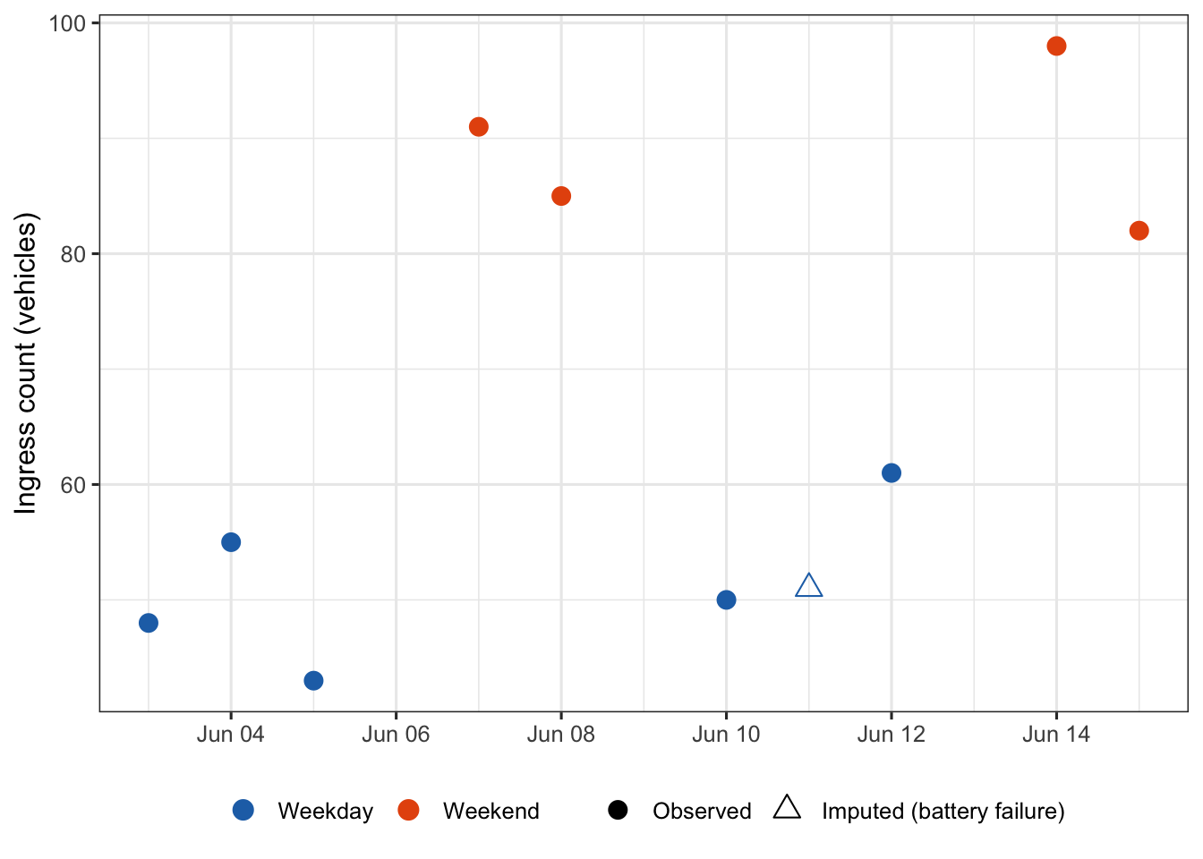
Weekday mean ingress on operational days is 51 vehicles; the imputed value for June 11 (weekday, battery failure) is 51 — the stratum mean. With more operational weekdays in the training set, the GLM would use day-of-week or environmental covariates if they were present in the data.
Figure 11.3 shows the ingress counts across the survey period, with the imputed observation visually distinguished.
Figure 11.3: Daily boat-ramp camera ingress counts over the survey period. Observed counts (solid points) are distinguished from the imputed value on June 11 (open triangle, battery failure). Weekend counts are consistently higher than weekday counts, reflecting the typical recreational fishing pattern.
Building the camera design
Camera designs use design_type = "camera" and require camera_mode to specify what the counter records. The current supported modes are:
"counter" — a simple ingress counter (vehicles or anglers entering)
"ingress_egress" — paired ingress and egress timestamps, from which preprocess_camera_timestamps() computes trip-level effort
The counter mode is the most common and requires only the imputed count table passed to add_counts(). This is the simplest camera case: the sensor gives a daily traffic total, and the analyst reconstructs angler-hours from counts and mean trip length.
Warning in svydesign.default(ids = psu_formula, strata = strata_formula, : No
weights or probabilities supplied, assuming equal probability
Warning: ! No `n_anglers` provided — assuming 1 angler per interview.
ℹ Pass `n_anglers = <column>` to use actual party sizes for angler-hour
  normalization.
ℹ If the interviews really are one angler each, pass `n_anglers = 1` to state
  that and silence this warning.
Warning: 14 interviews have zero catch.
ℹ Zero catch may be valid (skunked) or indicate missing data.
est_effort_camera() uses the ratio of mean interview trip duration to the camera count — a ratio estimator that converts ingress events to angler-hours. The intuition: if the camera records 60 vehicles entering and the mean trip length from interviews is 3.5 hours, the day-level effort is approximately 60 × 3.5 = 210 angler-hours. The ratio is estimated within strata and expanded to the full survey period:
Warning: 1 of 10 count days (10%) contains imputed counts.
✖ Prediction uncertainty for imputed counts is not included in the SE.
ℹ Imputed counts also vary less than observed ones, so the between-day
  component is understated as well; the reported SE is a lower bound.
Warning: Camera ratio calibration cannot tell angler-hours from party-hours.
✖ hours_fished is a caller-supplied column and nothing on this path normalises
  it by party size.
ℹ Pass `n_anglers` -- a column in `interviews`, or a constant party size -- to
  make the unit derivable.
ℹ The estimate is returned with an unknown unit until then.
Code
effort_camera
── Creel Survey Estimates ──────────────────────────────────────────────────────
Method: camera_ratio
Variance: Taylor linearization
Confidence level: 95%
Count-sampling SE: 4.182 (included in se)
Calibration SE: 10.12 (included in se)

# A tibble: 1 × 7
  estimate    se se_between se_within ci_lower ci_upper     n
     <dbl> <dbl>      <dbl>     <dbl>    <dbl>    <dbl> <int>
1     123.  10.9       10.9         0     97.9     148.    10
The result is a total angler-hours estimate with a Taylor-linearization standard error. For the example data, 123.1 angler-hours (95% CI: 97.9–148.3) across the 10-day window. The se_between component reflects between-day variation in the ingress × trip-length product; se_within reflects within-day interview variance in trip duration.
That split tells you where the next precision gain is likely to come from: more camera-days if between-day variation dominates, more interviews if trip-length variation dominates.
As with the aerial design, catch rate estimation is unchanged:
Code
estimate_catch_rate(design_camera)
ℹ Using complete trips for CPUE estimation
  (n=40, 100% of 40 interviews) [default]
── Creel Survey Estimates ──────────────────────────────────────────────────────
Method: Ratio-of-Means CPUE
Variance: Taylor linearization
Confidence level: 95%
Unit: fish/party-hour

# A tibble: 1 × 5
  estimate     se ci_lower ci_upper     n
     <dbl>  <dbl>    <dbl>    <dbl> <int>
1    0.453 0.0755    0.305    0.601    40
The design_type affects only how effort is estimated. From estimate_catch_rate() onward, camera and access-point designs use identical code paths.
Ingress-egress timestamps
When cameras record both arrival and departure times for individual vehicles, preprocess_camera_timestamps() converts the raw timestamp pairs into daily effort totals. This requires a data frame with one row per vehicle event and ingress_time and egress_time columns as POSIXct values:
The output is a daily summary of total recorded angler-hours from timestamp differences. This can substitute for or supplement the interview-based mean trip duration estimate — the camera itself measures effort directly, rather than inferring it from a count and a mean duration.
This is the cleanest camera case because effort is observed directly from the start and end times rather than inferred from counts.
11.4 Sample size for camera designs
Once a pilot camera season establishes the stratum-level mean and variance of the ingress × trip-length product, creel_n_camera() returns the number of sampled days needed to achieve a target coefficient of variation. The required inputs mirror those of creel_n_effort(): target CV, total days in the stratum, and stratum-level mean and variance from the pilot:
Code
# Compute stratum summary from operational days onlycam_summary <- camera_counts_clean |>filter(!.imputed) |>group_by(day_type) |>summarise(N_h =n(),ybar_h =mean(ingress_count),s2_h =var(ingress_count),.groups ="drop" )cam_summary
# Days needed per stratum to achieve CV = 0.15# creel_n_camera() requires named numeric vectorscreel_n_camera(cv_target =0.15,N_h =setNames(cam_summary$N_h, cam_summary$day_type),ybar_h =setNames(cam_summary$ybar_h, cam_summary$day_type),s2_h =setNames(cam_summary$s2_h, cam_summary$day_type))
  weekday   weekend     total allocated
        1         1         1         2
With only five operational weekday observations and four weekend observations, the variance estimate is too thin to say much, so both strata bottom out at n = 1. That is a toy-data artifact: real pilot seasons with 20–30 operational days per stratum usually provide enough spread in ingress counts to make the calculation informative. Treat the output as a minimum sample-size target for each stratum, not as a precise optimum. creel_n_camera() also emits a warning when the pilot falls below the empirical minimum recommended by Feltz and Middaugh (2025); that warning is suppressed here because the example data intentionally fall below it.
11.5 Proxy counts and validation
Vehicle counters and gate sensors
Aerial counts and camera-monitored ramps are the most thoroughly supported remote-count methods in tidycreel, but other proxy systems appear in practice: pneumatic road tubes at boat launch entrances, infrared gate sensors at trailheads, and acoustic hydrophone arrays that detect boat motors in restricted channels. Each records a correlated signal of fishing activity rather than a direct observation of anglers.
The key question for any proxy is how strongly it tracks what the survey domain requires. A pneumatic tube at a single-access boat ramp on a lake with no bank fishing likely correlates nearly 1:1 with launched boats. A road-tube counter at a multi-access reservoir where some anglers walk in from informal paths captures only the trailered-boat fraction. The correlation structure — and therefore the calibration factor — depends on access geometry, angler behavior, and whether the proxy integrates the full reporting domain.
Calibration against ground truth
Paired sampling is the standard validation approach: on a subset of days, both the proxy count and a direct ground count are collected on the same time window. The ratio of ground count to proxy count on paired days becomes the calibration factor applied to proxy-only days.
A calibration regression extends this: ground = a + b × proxy with the slope b estimated from paired days. The intercept accounts for baseline angler activity not captured by the proxy (walk-in anglers, for example), and the slope converts proxy units to ground-count equivalents.
Code
# Paired calibration: road-tube counter vs direct creel-crew count on the same days# Simulated paired data: 15 days where both methods were deployed simultaneouslyset.seed(42)paired_days <-tibble(date =seq.Date(as.Date("2024-06-03"), by ="2 days", length.out =15),tube_count =as.integer(rpois(15, lambda =55)),crew_count =as.integer(round(0.82* tube_count +rnorm(15, 0, 4))))cal_fit <-lm(crew_count ~ tube_count, data = paired_days)coef(cal_fit)
(Intercept)  tube_count
  2.1682712   0.8162411
The intercept (2.2) captures angler activity not counted by the road tube — walk-in anglers, kayak launches from an unmonitored site. The slope (0.816) converts tube-count units to crew-count equivalents. On proxy-only days, multiply the tube count by this slope and add the intercept to recover the calibrated angler count before applying mean trip length.
A slope near 1.0 indicates the proxy and direct count are on the same scale; a slope below 1 indicates systematic undercounting — the tube misses some fraction of the angler population — that the calibration corrects. The regression diagnostic (R^2, residual plot) should be checked before trusting the calibration: if the relationship is noisy or nonlinear, a simple ratio calibration will not transfer reliably to proxy-only days.
Documenting downtime and coverage gaps
No remote monitoring system has perfect uptime. Effective survey documentation requires a record of:
Days when the system was fully operational
Days with partial downtime (camera down for X of Y hours)
Days with complete failure (no data)
Known failure modes (battery, connectivity, vandalism, weather)
The camera_status column in example_camera_counts illustrates the minimum required record. In practice, richer downtime records allow the imputation model to condition on failure type — battery failures cluster by temperature and season; connectivity failures cluster by storm events.
A camera with 90% uptime over a 30-day survey loses roughly 3 operational days. If those failures are random relative to angler activity, imputation adds noise but not much bias. If failures correlate with weather — cameras fail in cold rain, which also suppresses fishing — the imputed values reflect low-use conditions, and the estimate is biased downward. Understanding the failure mechanism matters as much as the imputation method.
11.6tidycreel support summary
The three major remote-count workflows and their tidycreel entry points:
Design
design_type
Count function
Estimate function
Aerial GLMM
"aerial"
add_counts() (raw flights)
estimate_effort_aerial_glmm()
Camera counter
"camera"
add_counts() (imputed)
est_effort_camera()
Camera ingress/egress
"camera" + timestamps
preprocess_camera_timestamps()
est_effort_camera()
Proxy count (manual calibration)
any
calibration regression
ratio applied to standard estimate
All four share the same downstream pipeline: design object → add_interviews() → estimate_catch_rate() / estimate_total_harvest(). The remote-count method changes how effort is estimated; catch rate and harvest estimation proceed identically to access-point and roving designs.
11.7 Key considerations
Frame alignment. The camera or aircraft must cover the same spatial domain as the reporting unit. A ramp camera that misses an informal carry-in launch is not counting the full angler population. Aerial coverage that excludes a productive back bay leaves effort in that bay unrecorded. Frame gaps in remote designs are harder to detect than in creel-crew designs because there is no field crew to notice unexpected activity outside the monitored area.
Timing alignment. For aerial designs, h_open must match what the GLMM integrates over. If the model integrates from 06:00 to 20:00 (14 hours) but fishing in the reporting domain occurs only between 07:00 and 18:00, the integration window overestimates effort. Setting h_open conservatively from local sunrise-to-sunset tables avoids this bias.
Sensor resolution. A camera that counts vehicles counts launched boats (typically one to four anglers per boat). Converting vehicle counts to angler-hours requires an estimate of mean party size from interviews — an additional ratio estimator step with its own variance. The standard error from est_effort_camera() propagates this uncertainty automatically when party-size information is included in add_interviews().
Uptime documentation. Effort estimates from camera designs are only as reliable as the imputation model for failed days. More operational days in the calibration sample → better imputation. Effort estimates should report the fraction of days that were imputed alongside the estimate and standard error, so users can assess how much of the result rests on modeled versus observed counts.
Remote count designs extend the creel survey toolkit substantially: larger waterbodies become tractable, high-frequency temporal monitoring becomes affordable, and record-keeping becomes auditable. What they do not change is the need for a defined frame, a defensible sampling design, and explicit assumptions about what the sensor measures and what it misses.