creel survey, fisheries, design-based inference, R, tidycreel, Quarto
12.1 Purpose
A creel survey schedule is not just a list of days to work. It is a series of commitments about which parts of the fishery will be observed, how often, and in what proportion.
Stratification is the tool that makes those commitments explicit. By dividing the sampling frame into groups before drawing the sample, the analyst ensures that each part of the fishery contributes to the estimate in a controlled and defensible way. A poor stratification plan can weaken an estimate before a single angler is interviewed. A good one turns the heterogeneity of fishing use into a feature the estimator can exploit.
This chapter covers:
why strata are a design decision, not a reporting label;
the statistical logic connecting stratification to variance reduction;
how much stratification gains over simple random sampling, and when the gain is large;
common creel strata — temporal, spatial, and angler-type — and how to choose among them;
the minimum-samples-per-stratum constraint and when adding strata hurts;
how allocation strategy follows from the research question, not from formulas alone;
the low-use trap: why proportional allocation can create strata with undefined catch rates;
building a schedule with generate_schedule(), including high-use day handling;
generating and attaching count times with generate_count_times() and attach_count_times();
auditing stratum-level precision with audit_strata(); and
planning sample sizes with power_creel().
12.2 What stratification does
Stratification divides the sampling frame — the set of all eligible sampling units — into mutually exclusive groups called strata. Within each stratum a separate random sample is drawn. The final estimate combines stratum-level estimates using known weights derived from the design.
The practical motivation is almost always variance reduction. If the sampling frame contains groups that behave very differently from each other, pooling them into a single sample introduces unnecessary noise. A random sample drawn from a mixed population has to average over that heterogeneity. A stratified sample can represent each group directly, then combine with appropriate weights.
In creel surveys the dominant source of heterogeneity is usually temporal. Effort on a summer Saturday is not drawn from the same distribution as effort on a Tuesday in September. If both are included in an unstratified sample with equal probability, the estimate becomes sensitive to chance variation in which days happened to be selected. Stratification removes that sensitivity by guaranteeing that each day type is represented in proportion to its importance or its variance.
Stratification also protects the estimate against a subtler problem: silent misrepresentation. If weekends make up 30 percent of the season days but are accidentally undersampled, the final total will be biased toward weekday conditions. Stratification forces the analyst to state the day-type composition explicitly, which makes any deviation from the intended allocation immediately visible.
The scale of that heterogeneity also determines the right level of temporal resolution. Creel surveys operate on a three-stage sampling structure (Cochran 1977; Rasmussen et al. 1998): the first stage is the day, sampled by random selection within each stratum; the second stage is the shift within the sampled day; and the third stage is the count time within the shift. Each stage contributes its own component of variance to the total. Variance among days drives how many days to sample; variance within days across count times drives how many counts to take per shift. Newman et al. (1997) showed that the ratio of among-day variance to within-day variance governs the optimal trade-off between these two dimensions — when among-day variance is large relative to within-day variance, adding sampling days reduces total uncertainty more than adding count times within existing days.
Before modern computing made stratum-level estimation routine, the standard approach was to compute an “average day” for each month by weighting weekday and weekend mean values, then multiply that average by the total days in the month (Malvestuto 1996). The contemporary approach estimates means and variances separately for each stratum in each month, scales each to its stratum size, and sums across strata to produce the monthly total. The difference matters: the historical approach masked between-stratum contrasts and required implicit assumptions about their proportions; the stratified approach makes those proportions explicit and immediately auditable.
Important
A stratum is not a reporting label that can be added after the survey. The strata used for estimation must match the strata used for sampling. If a stratum was not explicitly part of the sampling design, its records cannot be weighted correctly.
12.3 The stratified estimator
Consider a season divided into H strata. Stratum h contains N_h sampling days, of which n_h are selected by simple random sampling. The population total is estimated as:
\hat{Y}_{st} = \sum_{h=1}^{H} N_h \bar{y}_h
where \bar{y}_h is the sample mean within stratum h. The variance of this estimator is:
The term (1 - n_h / N_h) is the finite population correction (FPC). It shrinks the variance when n_h approaches N_h — sampling a large fraction of the stratum leaves little uncertainty about what was not sampled.
Two properties of this expression matter for design decisions:
Variance depends on s_h^2, the within-stratum variance, not the between-stratum variance. Defining strata that are internally homogeneous reduces s_h^2 and therefore reduces the total variance.
The N_h^2 multiplier means that large strata dominate the total variance even when their within-stratum variance is modest. A high-use stratum that accounts for half the season days will drive the estimate’s uncertainty.
12.4 The gain from stratification
The justification for stratification rests on a formal comparison with simple random sampling (SRS). Under SRS with total sample size n, the variance of the total estimator is:
The quantity S^2 - \bar{S}_w^2 is the between-strata component of variance — how much of the total population variance is explained by differences in stratum means. Stratification eliminates between-strata variance from the estimator entirely. When weekday and weekend means differ substantially (a weekend mean of 110 anglers versus a weekday mean of 48), the between-strata component is large and the gain from stratification is substantial. When stratum means are similar, stratification provides little benefit and may introduce administrative complexity without reducing uncertainty.
Cochran (1977) showed that proportional allocation achieves its maximum benefit when strata are internally homogeneous — when the variation remaining within each stratum is small relative to the variation across the whole population. The gain depends entirely on the contrast between stratum means, not on their absolute magnitudes. Two strata with means of 40 and 120 anglers per day produce a larger variance reduction than two strata with means of 80 and 85, even if the higher-mean strata have larger absolute day-to-day variability.
Note
Stratification under proportional allocation always reduces or at worst equals SRS variance — it can never make estimates worse. Neyman allocation can reduce variance further, but it requires pilot estimates of s_h and can only be applied if those estimates are reliable.
12.5 Types of strata in creel surveys
Temporal strata
The most common creel strata divide the season by day type and by time period within the day.
Day type is the workhorse stratum. Weekend use is typically higher and has different species composition than weekday use. In most reservoirs and rivers, a design that treats all days identically would need a much larger sample to achieve the same precision as one that separates weekends from weekdays.
Holidays and high-use days add a third temporal stratum. Memorial Day weekend, the Fourth of July, and Labor Day can produce effort levels that are well above the normal weekend distribution. Collapsing them into the weekend stratum inflates weekend variance and risks over- or under-representing the most intense use of the season. When there is field evidence that holiday use differs systematically from ordinary weekends, a three-stratum design is worth the added complexity.
Shift divides the sampling day into morning and afternoon periods. Most creel designs treat the shift as a period nested within the sampled day rather than a separate stratum, but the distinction matters for how counts are expanded to a daily total.
Month or season segment is sometimes used when species composition or effort intensity changes across the season in predictable ways. Early and late-season strata are common in trout fisheries where opening day and late-summer conditions differ sharply.
Spatial strata
Large waterbodies or river systems can be divided spatially when different reaches or basins attract different fishing pressure or support different species assemblages. Spatial strata work like temporal strata in the estimator: each stratum contributes a separately weighted component to the total. The practical constraint is that spatial stratification multiplies field effort because each stratum requires its own sample.
Angler segmentation
Temporal and spatial strata divide the sampling frame in time and space. A third dimension — angler type — divides the sample by behavior. The most common segmentation distinguishes boat anglers from bank anglers, but other divisions appear when fishing methods or target species differ predictably across groups.
The justification is not administrative convenience. Boat and bank anglers use the water at different times of day, have different catch rates for most species, and have fundamentally different detection probabilities during an instantaneous count (Pope et al. in press). On most reservoirs, a count conducted at mid-morning will encounter all boat trailers in the parking lot but may miss bank anglers dispersed along a shoreline a kilometer from the ramp. If the sampling design does not account for this, effort estimates for bank anglers will be systematically low.
When angler groups differ in their fishing patterns, ignoring segmentation in the design introduces bias of unknown magnitude and direction — the direction depends on the actual ratio of boat to bank effort on specific sampled days, which the analyst cannot know in advance (Pope et al. in press). In practice, separate count and interview protocols for each group are combined at the stratum level: counts from each segment become effort estimates for each segment, and the interview records from each segment produce catch rates for each segment.
Segmentation can be omitted when only one behavior is present or when total effort summed across all behaviors is the only estimand. It becomes unavoidable when species-specific catch rates differ by angler type, when the research question targets behavior-specific outcomes, or when different access types (boat ramp versus bank access point) are spatially separated and sampled differently.
How many strata are enough?
Adding strata always reduces within-stratum variance — up to a point. Cochran (1977) showed that most of the gain from stratification is achieved with five or six strata; beyond that, the remaining within-stratum variance cannot be partitioned further without creating trivially small groups that are logistically unmanageable.
In creel surveys, the practical ceiling arrives sooner because of a hard constraint: every stratum requires a minimum of two sampled days to compute an estimate of within-stratum variance. Without that variance estimate, confidence intervals cannot be constructed. A design with four strata (weekday, weekend, high-use, early-season) and a monthly budget of 16 sampling days allocates 4 days per stratum at best under equal distribution — workable, but fragile. Any missed days due to weather or staffing can drop a stratum to one observation, which gives a mean but no variance and therefore no basis for a confidence interval.
Malvestuto (1996) recommended treating the two-sample minimum not as a statistical nicety but as a hard design constraint that precedes allocation decisions. Before choosing how many days to assign to each stratum, confirm that the proposed allocation satisfies the minimum for every stratum under realistic field conditions — not just the planned conditions. A stratum that regularly falls below two sampled days in the realized data is not a stratum the estimator can use reliably.
The test for whether a stratum is worth adding is whether the proposed division produces stratum means that differ practically. A month stratum that separates June from July but shows nearly identical mean daily effort in both may reduce within-stratum variance marginally but requires twice the administrative overhead. Prior data or a pilot season should establish that the proposed division captures a real contrast before the stratum is committed to the design.
12.6 Allocation strategies
Defining strata is the first decision. The second is how many sampling days to assign to each stratum.
Proportional allocation
The simplest approach assigns sample effort in proportion to the number of days in each stratum:
n_h = n \cdot \frac{N_h}{N}
Proportional allocation guarantees that each day in the season has an equal probability of selection. It is a reasonable starting point when little is known about stratum variances, but it does not minimize the total variance unless stratum variances happen to be equal.
Proportional allocation has a structural vulnerability in creel surveys: it assigns very few sampled days to low-use strata. On a reservoir where weekends account for 75 percent of season effort, proportional allocation assigns only 25 percent of the sample budget to weekdays. In a month with 22 eligible weekdays, a budget of 16 sampling days leaves weekdays with 4. Four days is a valid sample, but consider the consequence when those days have low use: if two of the four sampled weekdays have zero anglers present, the analyst has count data (a zero count, meaning zero effort) but no interview data — a catch rate that is undefined, not zero. The estimator cannot produce a catch total for that stratum and month because the catch rate is missing. Pope et al. (in press) noted explicitly that the agency must place a premium on variance estimates that cannot be satisfied with missing data, and recommended increasing weekday allocation beyond what proportional assignment would suggest.
This failure mode is distinct from a zero catch rate. A zero catch rate means anglers were present but caught nothing — a valid and usable observation. A missing catch rate means there were no anglers to interview on the sampled day. Only the latter creates an estimation failure; the former propagates normally through the estimator.
Optimal (Neyman) allocation
Neyman allocation minimizes total variance for a fixed total sample size:
n_h = n \cdot \frac{N_h s_h}{\sum_{k=1}^{H} N_k s_k}
Strata with larger standard deviations s_h receive proportionally more sample effort. In creel surveys this typically means the weekend stratum gets more days than proportional allocation would assign, because weekend effort tends to vary more from day to day — tournaments, weather, and holiday spillover all create high-variance weekend observations.
Neyman allocation requires a pilot estimate of each stratum’s standard deviation. These can come from prior surveys, agency data, or a short pilot season. Cochran (1977) provides the theoretical derivation; McCormick and Meyer (2017) applies it specifically to creel contexts.
Targeted allocation
When one stratum is management-critical — for example, the opening week of a trophy fishery — the analyst may oversample it relative to its size or variance. This is a deliberate departure from variance minimization in favor of reporting precision for a specific domain. The tradeoff is that the overall seasonal estimate may be less precise than under Neyman allocation, but the estimate for the targeted stratum will be more reliable.
Note
There is no universally correct allocation. The right choice depends on the reporting goal, the available field days, and prior knowledge of stratum variances. The formulas above clarify the tradeoffs; the decision still belongs to the analyst.
What the research question decides
No allocation formula substitutes for clarity about what the survey must produce. The three strategies above represent points on a spectrum from “represent the fishery proportionally” to “minimize overall uncertainty” to “maximize precision for a targeted domain.” All three are defensible; the choice depends on what the agency needs to report and to whom.
An annual harvest report requiring defensible stratum-level estimates for each month and day type needs at least two sampled days in every stratum — which means Neyman allocation cannot reduce any stratum to fewer than two days, regardless of what the formula returns. A seasonal total estimate tolerates higher stratum-level uncertainty in exchange for fewer total sampling days. A management study focused on a specific event — the first two weeks of a walleye season or a post-stocking period (Harmon et al. 2018) — may deliberately oversample that window at the cost of weaker estimates for the remainder.
A useful discipline: write the reporting tables first, then design the strata that will fill them. If the final report must present a 95 percent confidence interval for weekend catch by month, the weekend stratum must have enough sampled days per month to support that interval. If the report only needs a seasonal total, monthly strata may be unnecessary. The strata exist to serve the estimand, not the other way around.
12.7 Building a schedule
generate_schedule() produces a stratified random sampling calendar for a survey season. The function classifies every date in the season as weekday or weekend, randomly selects the requested number of days within each stratum, and expands the output to one row per sampled day per sampling period.
Basic two-stratum schedule
The simplest case uses two strata and specifies the number of days to sample in each:
Each row is one period on one sampled day. The day_type column carries the stratum assignment. The period_id column identifies the shift within the day.
The seed argument makes the schedule reproducible. A creel schedule is part of the study’s permanent record — the same seed should be used every time the schedule is regenerated from the same inputs.
Sampling rate specification
When the total number of days to sample is not fixed, sampling_rate expresses the fraction of each stratum to sample:
A higher sampling fraction for weekends reflects the fact that weekend variance typically drives overall uncertainty. n_days and sampling_rate are mutually exclusive — supply one or the other.
Adding high-use strata with special_periods
Holidays require a third stratum. The special_periods argument accepts a data frame that reassigns specific date ranges to a new stratum label before days are sampled. This happens before sampling, so holiday days are drawn separately from the baseline weekend pool.
The final_stratum column shows the resolved stratum after holiday reassignment. The special_period_reason column records why each date was reclassified — useful when the schedule is reviewed months later by someone who was not involved in the original design.
Tip
Holiday windows that cross month boundaries are handled correctly. A Labor Day weekend spanning August 31 to September 2 will not be split across two calendar months in the schedule.
12.8 Visualizing the schedule
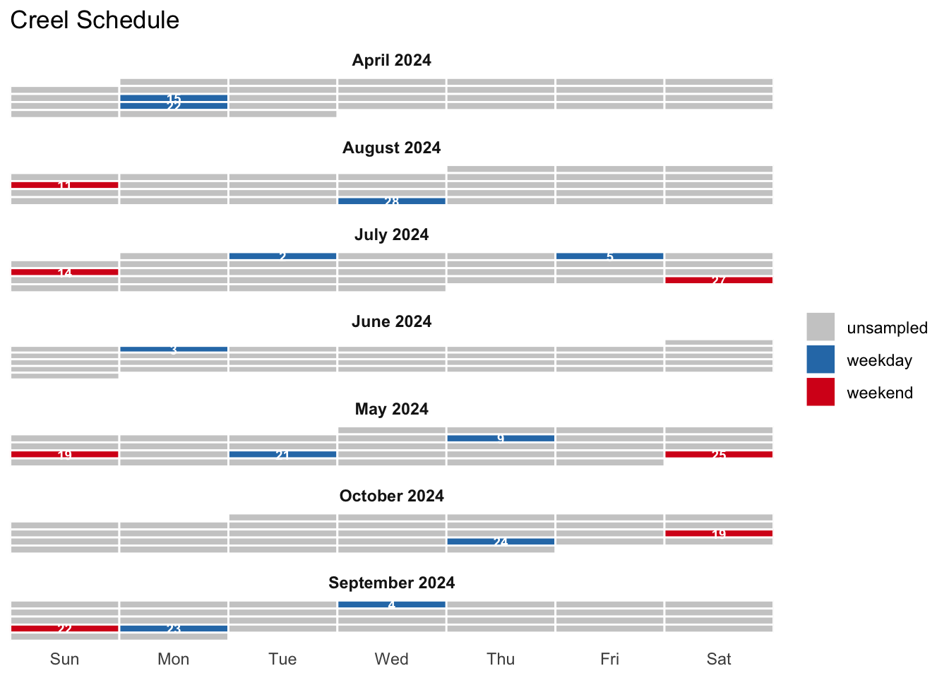
autoplot() produces a calendar-style view of the sampling schedule, with sampled days marked by stratum:
Code
autoplot(sched_hu)
Figure 12.1: Sampled days for a seven-month creel season on a reservoir with weekday, weekend, and high-use strata. Each colored cell represents one sampled day. The three-stratum structure ensures that holiday use patterns are estimated separately from ordinary weekend use.
This figure belongs in any report that includes creel estimates. It makes the coverage of the design immediately visible: which months were sampled heavily, which days of the week were prioritized, and whether the holiday stratum captured the intended calendar dates.
12.9 Generating and attaching count times
An instantaneous count is only unbiased if the time at which the count is made is selected randomly within the shift. generate_count_times() produces a set of count windows for a shift, and attach_count_times() joins those windows to the schedule so that each sampled shift knows when its counts are due.
Generating count windows
A standard morning shift runs from 06:00 to 14:00 — eight hours. To place three independent counts within that shift, divide it into three equal segments and sample one time within each:
Each row is one count window: a start time and end time during which the clerk completes an instantaneous count. window_size is the number of minutes allocated to the count itself (here 20 minutes per count). min_gap ensures that consecutive counts are separated by at least 60 minutes, preventing back-to-back observations that would not be independent.
Afternoon shifts use the same strategy with different boundaries:
The cross-join applies the same window specification to every period in the schedule. In a two-period design, morning and afternoon periods would each receive their own count window object generated with the appropriate shift boundaries. The full schedule, with count times attached, becomes the field crew’s daily reference document. write_schedule() exports it to CSV or XLSX for distribution to clerks.
12.10 Auditing stratum precision
After a pilot season or at the end of a survey, audit_strata() computes per-stratum RSE (relative standard error), design effect (DEFF), and a flag indicating whether each stratum meets the target precision.
Using pilot estimates
When pilot count data are available as summary statistics, call audit_strata() directly with the stratum means and variances:
Consider a pilot season spanning April through September on a mid-sized reservoir. The season contains approximately 130 eligible weekdays, 52 weekends, and 8 high-use holiday days. The pilot sample covered 24 weekday, 12 weekend, and 3 high-use days:
A stratum with meets_target = FALSE is under-sampled relative to its variance. The DEFF column compares each stratum’s contribution to the variance against what simple random sampling of the same total size would have produced.
The aggregate design effect across all strata is:
Code
pilot_audit$deff
[1] 0.7767957
Interpreting the audit
From the pilot output:
The weekday stratum meets the 20% RSE target comfortably. Its DEFF below 1.0 confirms that stratification reduced variance relative to an unstratified sample — the weekday distribution is internally homogeneous.
The weekend stratum also meets the target but has a DEFF well above 1.0. Weekend effort is more variable day-to-day; the stratum is contributing disproportionately to total uncertainty relative to an equal-probability design.
The high-use stratum fails the target (RSE = 0.26 > 0.20) and has a dramatically elevated DEFF. Three sampled holiday days provide almost no reliable estimate of what is often the most extreme effort of the season.
A DEFF below 1.0 at the aggregate level (the pilot_audit$deff output above) indicates that the overall stratification still improved on an unstratified design. But the stratum-level picture reveals where the next sampling investment should go.
12.11 Sample size planning
power_creel() with mode = "effort_n" uses pilot statistics to calculate how many sampling days each stratum needs to achieve a target RSE. This is the primary tool for converting an audit finding into a revised allocation plan.
Using the same pilot statistics from the reservoir example:
The n_required column gives the minimum sampling days under optimal (Neyman) allocation. The "total" row is the season-level field commitment.
The pilot sample covered 24 weekday, 12 weekend, and 3 high-use days. Comparing to the required plan: the weekday stratum is over-sampled relative to what the variance warrants; the high-use stratum’s allocation warrants careful review before committing to a main survey design, since a one-day sample cannot estimate within-stratum variance at all.
Warning
n_required = 1 for any stratum is a mathematical floor, not a practical recommendation. A minimum of two sampled days per stratum is required to estimate within-stratum variance — which is necessary for computing confidence intervals. If the high-use stratum has only a handful of eligible days in the season (here N_h = 8), the finite population correction makes the theoretical required sample small, but the practical minimum remains two days.
Proportional versus optimal allocation
Proportional allocation distributes sample effort in proportion to stratum size, while Neyman allocation weights by both size and variance:
Stratum
N_h
s_h
Proportional (n=30)
Neyman (n=30)
Weekday
130
30
~20
~14
Weekend
52
65
~8
~12
High-use
8
148
~1
~4
The high-use stratum has the largest per-day standard deviation by far. Neyman allocation shifts days toward it from the weekday stratum. Proportional allocation would give high-use the fewest days even though it drives the most uncertainty per observation. This table illustrates why the default assumption — “sample proportionally to size” — is often wrong for creel surveys where day-to-day variance is highly unequal across strata.
12.12 Planned versus realized allocation
The schedule produced by generate_schedule() is a plan. Weather, staff illness, road closures, and equipment failures will produce a realized sample that differs from the plan.
These deviations matter for two reasons:
The realized sample, not the planned sample, determines the estimate. If the design called for 6 weekend days in May but only 4 were completed, the estimate uses 4.
If the deviations are non-random — for example, bad weather consistently cancels Saturday counts — the realized sample may be biased even when the original plan was valid.
audit_strata() can be run on realized data from a completed design object. Comparing the realized RSE to the target RSE identifies which strata were under-served and flags whether a follow-up sample would be warranted.
What tidycreel cannot do is decide whether a missed day should be treated as missing at random or whether it reflects a systematic gap that biases the estimate. That judgment requires knowledge of why the day was missed, which only the field crew and the analyst together can provide.
12.13 Takeaway
Stratification determines how observations represent the fishery. The design question is not how many strata can be named, but which distinctions are worth their own sample.
In practical terms:
Define strata that reflect how anglers actually use the water — not how the calendar makes scheduling convenient.
Write the reporting tables before choosing allocation strategy; the strata exist to produce the estimands the report requires.
Give every stratum at least two sampled days; a stratum with one observation has no variance estimate and cannot support a confidence interval.
Account for angler-type segmentation (boat vs. bank) when detection probabilities or catch rates differ between groups — otherwise effort and catch estimates can be biased in unknown direction.
Remember that proportional allocation under-samples low-use strata, risking missing catch-rate data that produces undefined rather than zero estimates.
Use generate_schedule() with special_periods to handle holiday days that belong in their own stratum.
Use generate_count_times() to randomize counts within each shift, not fix them at convenient hours.
Use audit_strata() after a pilot season to identify which strata are under-sampled before the main survey begins.
Use power_creel(mode = "effort_n") to convert that audit into a revised allocation plan.
A well-stratified design spends sample effort where the fishery is most variable and most important, makes the reporting goals visible through the strata structure, and ensures that every component of the estimate can be checked against a clearly stated design decision.
Cochran, W. G. 1977. Sampling techniques, 3rd edition. John Wiley & Sons, New York.
Harmon, B. S., D. R. Martin, C. J. Chizinski, and K. L. Pope. 2018. Variation in angler distribution and catch rates of stocked rainbow trout in a small reservoir. PLOS ONE 13(1):e0190745.
Malvestuto, S. P. 1996. Sampling the recreational creel. Pages 591–623 in B. R. Murphy and D. W. Willis, editors. Fisheries techniques, 2nd edition. American Fisheries Society, Bethesda, Maryland.
McCormick, J. L., and K. A. Meyer. 2017. Sample size estimation for on-site creel surveys. North American Journal of Fisheries Management 37:970–980.
Newman, S. P., P. W. Rasmussen, and L. M. Andrews. 1997. Comparison of a stratified, instantaneous count creel survey with a complete mandatory creel census on Escanaba Lake, Wisconsin. North American Journal of Fisheries Management 17:321–330.
Pope, K. L., C. J. Chizinski, A. J. Lynch, and J. R. Post. in pressin press. Creel surveys.
Rasmussen, P. W., M. D. Staggs, T. D. Beard, and S. P. Newman. 1998. Bias and confidence interval coverage of creel survey estimators evaluated by simulation. Transactions of the American Fisheries Society 127:469–480.