creel survey, fisheries, design-based inference, R, tidycreel, Quarto
15.1 Purpose
Not every creel problem is an estimator problem.
The chapters that follow this one build estimators for effort, catch, harvest, and CPUE. Those estimators are correct — in the sense that they are unbiased and consistent — given certain conditions. The conditions include a well-constructed sampling frame, a protocol that was actually followed, and an interview process that sampled anglers at random without systematic exclusions.
When those conditions fail, no estimator fixes the result. A variance formula does not recover anglers who were never in the frame. A smarter catch-rate estimator does not undo the effect of a protocol that only interviewed cooperative anglers. An elegant ratio estimator cannot produce an unbiased total from a survey that missed three weeks of peak summer fishing.
This chapter names the most common ways creel surveys go wrong before estimation ever starts. The goal is to give analysts a vocabulary for diagnosing what happened, communicating it honestly, and deciding whether the problem belongs in field operations, frame construction, or the limitations section of the report.
15.2 A taxonomy of creel survey error
Creel survey errors fall into two broad categories: bias and variance. Variance is the sampling variability that shrinks with more observations; it is managed through design choices like stratification and allocation. Bias is systematic error that does not shrink with more observations. Adding more interviews in the wrong place does not fix a coverage gap.
Within bias, the literature identifies several recurring types (Pollock et al. 1994):
Table 15.1: Taxonomy of creel survey errors, with detection and correction status. Coverage errors are the most dangerous because they are invisible in the data.
Error type
Source
Detectable from data alone?
Correctable in analysis?
Coverage
Frame misses a portion of the target population
No
No — missing group left no records
Nonresponse
Refusers differ from participants in measured variables
Partially — if refusals logged
Yes — with inverse-response-rate weights
Avidity
More-frequent anglers intercepted more often
Partially — trip length distribution
Partially — harmonic mean for roving; not for access-point seasonal frequency
Temporal
Survey does not cover full season or fishing day
Partially — schedule completeness
No — unsampled periods cannot be imputed without auxiliary data
Spatial
Some locations sampled more intensively than design specifies
Partially — effort mismatch by site
Partially — post-stratification if auxiliary counts available
Operational
Execution errors: missed shifts, data entry, selective interviewing
Yes — if records exist
Partially — removable if flagged early
The practical distinction that matters most is between structural problems (baked into the design) and operational problems (arising from how the design was executed). Structural problems require a redesign; operational problems can often be addressed in the next field season or caught during data cleaning.
15.3 Coverage bias
Coverage bias is the most consequential form of creel error because it cannot be detected from the data alone. If a category of angler was never in the frame, there are no records of them — no flags, no missing values, no anomalous numbers. The data look complete because the frame says they are complete.
Spatial coverage gaps
Access-point creel surveys define the sampling frame as a set of public boat ramps, fishing piers, and access sites. Any angler who reaches the water through a private dock, a club launch, or shoreline access on private land is outside that frame. If those anglers differ in their catch rates, species targets, or effort levels, the survey estimates are biased toward the public-access population.
The magnitude of the bias depends on the proportion of effort that moves through private access. On heavily developed lakes with extensive private waterfront, the excluded population may be substantial. On reservoirs with limited public access managed by a single agency, the frame coverage may be near complete.
The Harlan Reservoir survey covers public boat ramps at the reservoir’s four primary access points. Bank anglers at public shoreline areas are included in the interview protocol. The frame excludes:
anglers using private docks on the upper reservoir arms;
shore fishing on the restricted Corps of Engineers management zones;
anglers who access the spillway from the north road, which is seasonally gated.
These exclusions are not recorded in the data. They appear only in the survey design documentation, so an analyst working from the data file alone would not know they existed.
Temporal coverage gaps
The Harlan schedule covers two daily periods: a morning period of eight hours (Period 1) and an afternoon period of six hours (Period 2). Together these periods cover daylight fishing from shortly after sunrise to approximately one hour before sunset. Fishing activity that occurs before Period 1 begins, after Period 2 ends, or on days not sampled is outside the temporal frame.
For most reservoir fisheries in the continental United States, this exclusion is small. Nighttime fishing represents a minor fraction of total effort on most waters, and dawn activity is partially captured by the morning period. But on some fisheries — catfish impoundments, walleye lakes, ice fisheries — a survey that ends at dusk misses the most active portion of the day.
The Harlan schedule was designed to cover the peak activity window for the target species assemblage (Largemouth Bass, Walleye, White Bass). Catfish are present and fished nocturnally, but are not the survey’s primary target. This is an explicitly scoped exclusion, not an oversight.
What data validation does and does not tell you
tidycreel provides validation_report() to check raw data tables for structural problems: column types, missing values, out-of-range dates, and negative counts. Running it on the Harlan data shows all checks passing:
This is a reassuring result. It means the data are internally consistent — no impossible values, no structurally missing fields, no dates outside the survey window. But it does not mean the frame is complete. The function checks what is in the data; it cannot check what was never recorded.
A clean validation report rules out operational data errors. It does not rule out coverage gaps that were already built into the sampling frame.
15.4 Nonresponse bias
An angler who is approached for an interview but declines to participate is a refusal. An angler who cannot be interviewed because they have left the site, are driving, or do not speak the survey language is unable to answer. Both contribute to nonresponse.
Nonresponse is not a problem in itself. Most creel surveys expect some fraction of anglers to decline, and a 10–15% refusal rate is typical for well-conducted access-point surveys (Pollock et al. 1994). The problem is nonresponse bias: if anglers who refuse differ from anglers who accept in the variables being measured, the survey estimate is biased.
The most plausible direction of that bias in a creel context is upward pressure on catch rates. Anglers who had an unsuccessful trip may be more likely to wave off the interviewer and leave quickly. Successful anglers, with fish to show and a story to tell, are more likely to linger. If this pattern holds, the interview sample overrepresents catching parties and overstates CPUE.
The opposite pattern is also possible. Avid anglers who fish frequently may grow weary of being interviewed on every visit and begin declining. If avid anglers catch at higher rates, repeated refusal from that group biases the estimate downward. The direction of bias is not knowable from the data alone.
Tracking refusals in a creel design
When the field protocol records refusals — a refused-interview log separate from completed interviews — tidycreel can tabulate them by month:
Warning: ! No `n_anglers` provided — assuming 1 angler per interview.
ℹ Pass `n_anglers = <column>` to use actual party sizes for angler-hour
  normalization.
ℹ If the interviews really are one angler each, pass `n_anglers = 1` to state
  that and silence this warning.
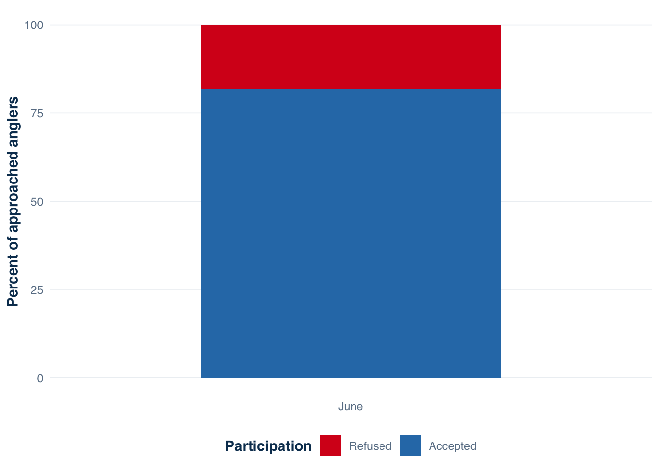
Figure 15.1: Interview participation rate by month. Each bar shows the fraction of approached anglers who accepted (dark) or refused (light) an interview. Refusal rates above 20% warrant investigation into whether refusers differ systematically from participants.
A refusal rate near 18% across the survey (as in Figure 15.1) is within the typical range for an access-point design, but it is not negligible. Before treating the estimate as representative, an analyst should ask whether crews recorded any systematic patterns — time-of-day clusters, specific access points with higher refusals, or demographic patterns in who declined.
Correcting for nonresponse with weight adjustments
When refusal data are available by stratum, adjust_nonresponse() applies an inverse-response-rate weight correction within each stratum. The function rescales survey weights so that the responded fraction represents the full approached population, not just the participants:
The weight adjustment inflates the contribution of each completed interview to compensate for the fraction that refused. A weekday response rate of 84% produces a weight multiplier of 1.18; a weekend response rate of 80% produces 1.25. When these adjustments are applied, downstream calls to estimate_catch_rate() or estimate_effort() on the adjusted design automatically incorporate the corrected weights.
The correction assumes that respondents and nonrespondents are similar within each stratum. If that assumption fails — if, say, weekend refusers include a disproportionate share of anglers who caught nothing — the adjusted estimate is still biased, just less so than the unadjusted version. Nonresponse weighting reduces, not eliminates, the problem.
The Harlan 2022 survey did not record refusals. The adjustment workflow is presented here using constructed response rates for illustration. For a future season, recording refusals requires only adding a boolean field to the clerk’s data entry form and passing refused = "refused" in add_interviews().
15.5 Avidity bias
Avidity bias arises from a mismatch between the design goal — a representative sample of fishing trips — and the sampling mechanism — intercepting anglers who are present at an access point at the moment of a survey shift.
An angler who fishes 40 days per season has 40 chances to be intercepted. An angler who fishes two days per season has two chances. If the two anglers differ in their catch rates, species preferences, or trip length, the sample overrepresents the avid angler. The survey sees the fishery through the eyes of its most committed users.
This is distinct from length-of-stay bias (also called size-biased sampling). On a roving survey, longer trips are more likely to be in progress during a transect pass. On an access-point survey, the mechanism is different: frequent-visitor anglers accumulate exposure across the season rather than within a single visit. Both produce an oversample of anglers who engage more intensively with the fishery (see the roving creel chapter for the harmonic-mean correction that addresses length-of-stay bias).
Trip length distribution
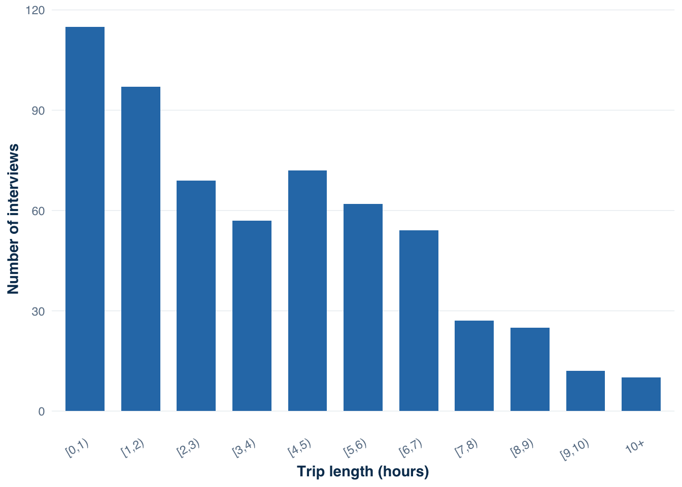
The distribution of completed trip lengths is informative about the likely direction of avidity bias. When the distribution is heavily right-skewed — most trips are short, but a long tail of multi-hour trips dominates angler-hours — the sample may be driven disproportionately by the long-trip segment.
Figure 15.2: Distribution of completed trip lengths at Harlan Reservoir, 2022. Most interviews record trips of under three hours, but the tail of four-to-nine-hour trips contributes a disproportionate share of total angler-hours and is more likely to be intercepted during a survey period.
Figure 15.2 shows that the Harlan sample is dominated by short trips. The modal bin is zero to one hour; more than 35% of completed interviews record trips under two hours. This is consistent with a reservoir where many anglers stop for an evening hour after work, or for a brief morning session before other commitments. A survey that covers eight-hour morning periods captures the full range of these trip lengths, including the long-tail anglers who started before the survey shift began.
The implication for avidity bias depends on whether trip length correlates with catch. For Walleye — which bite most actively at dusk and dawn — a short trip in the middle of the day may yield very different results than a full-day outing. The distribution itself does not prove bias, but it identifies where to look.
Angler type patterns across the season
Avidity patterns are not static. The composition of who uses a fishery shifts with species seasonality, weather, and regulations. A survey that is evenly spaced across the season will still see different populations in different months.
       month angler_type   N percent
1      April        bank  18    85.7
2      April        boat   3    14.3
3        May        bank 143    72.2
4        May        boat  55    27.8
5       June        bank  53    47.3
6       June        boat  59    52.7
7       July        bank  40    44.4
8       July        boat  50    55.6
9     August        bank  14    16.5
10    August        boat  71    83.5
11 September        bank   6    10.5
12 September        boat  51    89.5
13   October        bank   4    10.8
14   October        boat  33    89.2
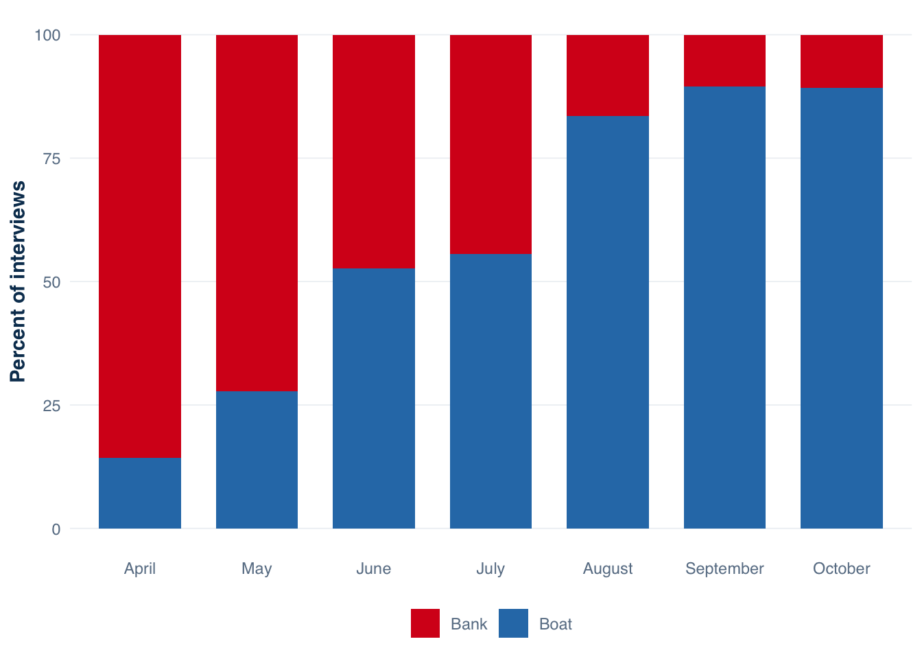
Figure 15.3: Composition of boat and bank anglers in the Harlan Reservoir sample by month. The shift from bank-dominated spring fishing to boat-dominated late summer reflects species-driven movement patterns: bank anglers target structure species in cool months; boat anglers follow Walleye and White Bass into open water as temperatures rise.
At Harlan, boat anglers increase from 14% of the spring sample to nearly 90% by late summer. This reflects the seasonal transition from bank-accessible structure fishing in April to open-water trolling for suspended Walleye and White Bass later in the year. A summary across all months treats the spring bank-fishing population and the late-season boat-fishing population as interchangeable, which they are not.
If boat and bank anglers differ in their catch rates, pooling them without stratification on angler type overstates the homogeneity of the fishery. Whether that pooling constitutes bias depends on the estimand: if the goal is the reservoir total, pooling is acceptable; if the goal is a per-trip comparison by method, it is not.
When avidity bias matters most
Avidity bias is most consequential in three situations:
Off-site diary and mail surveys — where participation is voluntary and avid anglers are far more likely to enroll (Pollock et al. 1994). On-site creel surveys are less exposed to this because interception is tied to presence, not to willingness to complete a mail questionnaire.
Roving surveys without harmonic-mean correction — where longer trips are proportionally overrepresented within a single shift. The roving creel chapter describes the harmonic-mean correction that addresses this specific mechanism.
Estimates reported at the angler level rather than the trip level — such as per-angler season harvest. The survey samples trips, not anglers. Inferring per-angler averages from trip-level data requires assuming that every angler has the same number of trips — an assumption that avidity bias directly violates.
For the Harlan access-point survey, avidity bias within a single survey period is not a primary concern because the estimator counts angler-hours rather than weighting by individual-level fishing frequency. Across the season, the concern is whether the mix of anglers in any given stratum is representative of the full population that fishes Harlan, including those who only visited on days that were not sampled.
15.6 Temporal coverage gaps
A survey can be correctly designed and carefully executed and still miss the fishing that matters most for an estimate.
The most common form of temporal undercoverage is unsampled days. A stratified schedule samples a fraction of available weekdays and weekend days in each month. The days that were not sampled may or may not resemble the days that were. In a stable fishery with slow-changing conditions, the unseen days are likely similar to the sampled days. After a significant weather event, a holiday weekend, or a tournament draw, they may not be.
A second form is within-day gaps due to shift structure. The Harlan schedule covers Period 1 (morning, eight hours) and Period 2 (afternoon, six hours). Fishing that begins after Period 2 ends is not captured. For species with strong crepuscular activity patterns, a design that does not extend into evening hours is structurally incomplete for those species.
A third form is fair-weather bias: surveys are more likely to be cancelled or shortened during rain, cold snaps, or high wind. If poor weather suppresses fishing (or changes who fishes and what they catch), then sampled days disproportionately represent favorable conditions. This inflates effort estimates if anglers fish less in bad weather, or distorts catch composition if weather-tolerant anglers target different species than fair-weather anglers.
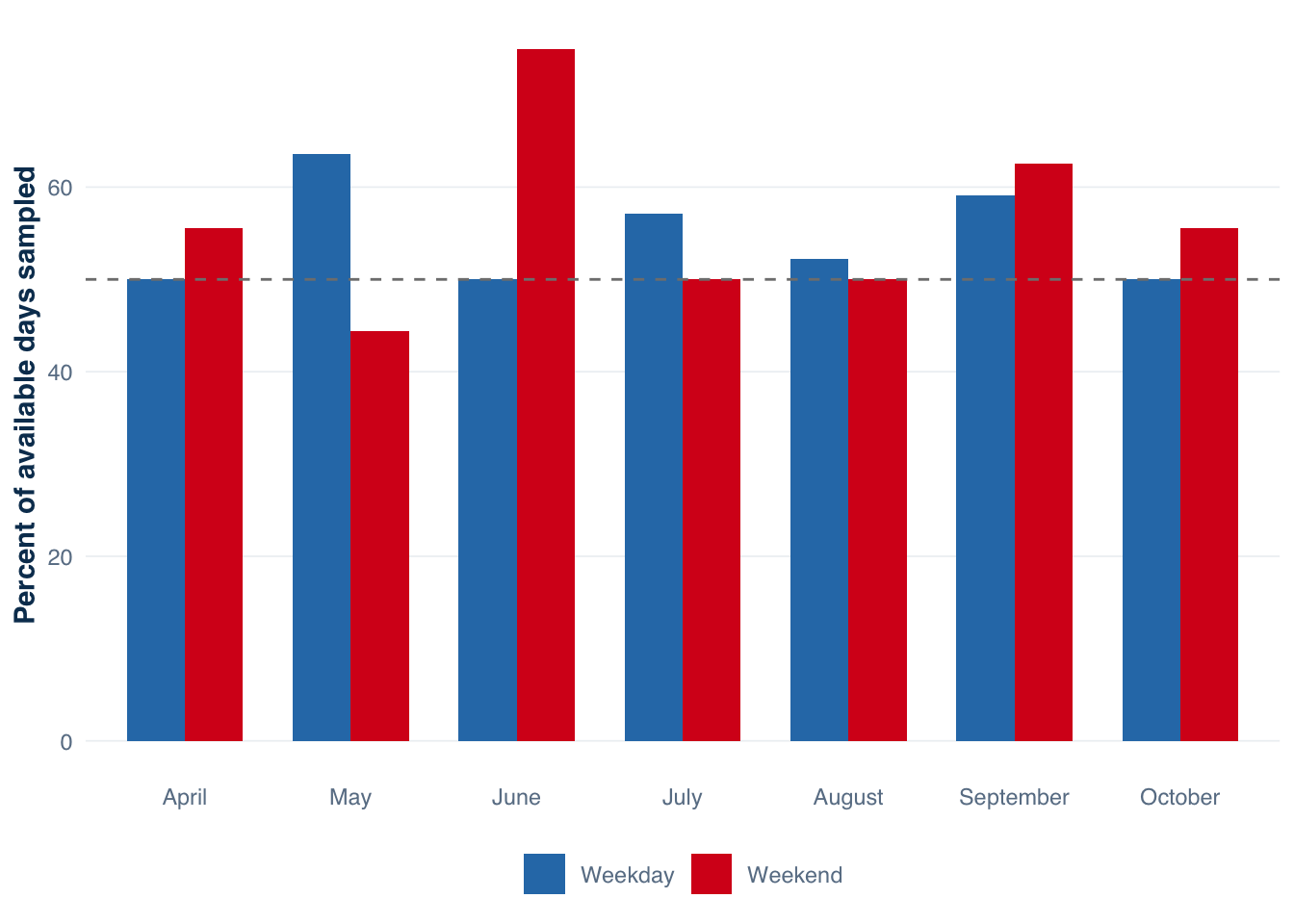
The schedule itself shows what proportion of available days were actually sampled in each stratum:
Figure 15.4: Harlan 2022 sampling coverage by month and day type. Each bar shows the fraction of available calendar days in that stratum that were included in the survey schedule. Coverage ranges from 44% to 75%, reflecting the stratified random draw from available weekday and weekend slots.
Figure 15.4 shows coverage near 50% for most month-stratum combinations, as expected from the stratified random draw. The June weekend stratum is the highest at 75%; the May weekend stratum is the lowest at 44%. These differences are within the normal range of a single-season sample — no stratum is missing or collapsed.
The Harlan 2022 field record does not include a log of cancelled or shortened shifts within sampled days. Without that record, it is impossible to assess whether fair-weather bias affected the estimates within the sampled shifts. For future survey seasons, logging each planned shift as completed, shortened, or cancelled — and recording the reason — takes five minutes per shift and makes the within-day temporal coverage audit tractable.
15.7 Operational failure modes
Operational problems differ from structural bias in that they arise from execution, not design. They are often visible in the data if analysts look for them early in the season rather than after the data are already collapsed into summaries.
Selective interviewing
The most common interviewing error is one that is not recorded as an error at all: interviewing only anglers who caught fish, or avoiding parties that appear unwilling to stop. Both patterns bias catch and CPUE estimates upward.
The simple audit is to compare the zero-catch rate in the interview data against the expected fraction based on local knowledge of the fishery. If the fishery is known to be difficult — a walleye impoundment in midsummer, say — but 90% of interview records show nonzero catch, selective interviewing is the likely explanation.
The Harlan data validate cleanly on this dimension: 318 of 600 total interviews (53%) recorded zero catch, which is consistent with observed conditions at a mixed-species reservoir in a moderate-productivity year.
Data entry errors
Recording errors at the field level — wrong species codes, transposed digits in angler counts, ambiguous trip status records — can introduce bias if they are not random. A pattern of systematic overrecording of fish counts (a clerk who rounds up, or who transcribes the number of fish in the cooler rather than the number reported by the angler) produces upward bias across the whole dataset.
Section 20.1 covers the flag_outliers() and standardize_species() tools for detecting and correcting these errors. The cleaning and the bias assessment are linked: if flag_outliers() turns up a cluster of anomalously large catches all recorded by the same clerk on the same set of dates, that is an operational failure, not random variation.
Species misidentification
Angler-reported species identification is unreliable when species look alike, when anglers are targeting one species and incidentally catching another, or when field staff lack experience with local species assemblage. Page et al. (2012) estimated that species misidentification in an Ohio reservoir survey inflated catch estimates for some species by up to 386%. The effect on a total-catch estimate depends on whether misidentification is symmetric (random swaps between species) or directional (consistently misidentifying a less common species as a more common one).
standardize_species() detects codes that do not match the AFS species list, which catches typographical errors and nonstandard abbreviations. It does not catch biologically plausible misidentifications — a Walleye recorded as a Sauger, or a White Bass recorded as a Striped Bass. Those require species-specific diagnostic plots and cross-checking with electrofishing or netting records if they are available.
15.8 Structural versus operational problems
The distinction between structural and operational problems determines what can be fixed and when.
Structural problems are built into the design before any data are collected. They include:
Frame construction decisions that exclude a portion of the target population (private access, geographic restrictions, nocturnal exclusion)
Estimand misspecification — a survey designed to estimate platform-specific effort that is later asked to estimate species-specific totals it was not designed to support
Stratum definitions that cannot be collapsed or expanded to produce usable estimates in thinly sampled sub-periods
These problems cannot be fixed by cleaning the data, choosing a better estimator, or adding covariates. The frame sets the population to which estimates can be validly generalized. An estimate made from a frame that excluded 20% of effort is an estimate for the 80% of effort that was in scope, even if the report is presented as if it covers the full fishery.
Operational problems arise from imperfect execution of a sound design:
Missed shifts due to staffing, weather, or equipment
Recording errors by inexperienced clerks
Departures from the random sampling protocol during busy periods
Species misidentification at the field level
Operational problems can sometimes be partially corrected in analysis — by removing anomalous records, imputing missing counts from similar dates, or weighting by response rate — but only if the problem is detected early enough. An operational problem discovered three months after the season ends, after field staff have moved on, is much harder to address than one caught in week two of the survey.
The field log and the data QC pass are the primary detection tools for operational problems. Neither the validation report nor the outlier flags in Section 20.1 can catch a problem that was not recorded. A shift that was cancelled but recorded as completed, or a set of interviews collected by a clerk who only approached fishing parties, leaves no visible trace in the data.
15.9 What tidycreel can and cannot fix
tidycreel provides a set of tools that address specific, diagnosable forms of bias — and that are honest about what they cannot address.
Can detect and correct:
Data entry errors and structural column problems (validation_report(), validate_creel_data())
Outliers in effort and catch that may indicate recording errors (flag_outliers())
Species code mismatches and nonstandard abbreviations (standardize_species())
Nonresponse bias, when refusals are recorded (summarize_refusals(), adjust_nonresponse())
Avidity bias within a single trip, for roving surveys (estimate_catch_rate(estimator = "mortr"))
Cannot detect or correct:
Coverage gaps: anglers outside the sampling frame generate no records
Selective interviewing that was never flagged in the field
Structural estimand mismatches between what was designed and what is being asked
Fair-weather bias when the field log does not record which shifts were cancelled
Species misidentification that is biologically plausible
The practical implication is that bias assessment must happen in two places: in the field log and design documentation (structural review), and in the data (operational review). A clean validation_report() rules out the second category. It says nothing about the first.
15.10 Diagnostic questions for analysts
When reviewing a creel estimate or preparing to report one, the following questions help locate the likely sources of remaining error:
Frame coverage: - Does the access point list include all sites used by the target population? - Are there modes of access (private launches, shoreline access, seasonal access roads) that were excluded? - Does the temporal schedule cover the full fishing day for the target species?
Nonresponse: - Were refusals recorded? What was the refusal rate by month, by time of day, and by access point? - Is there any evidence that refusers differed from participants (field notes, clerk observations)? - Was adjust_nonresponse() applied? If not, is that choice defensible given the refusal rate?
Avidity: - Is the survey design access-point or roving? Roving designs require additional correction for length-of-stay bias. - Does the trip length distribution show a heavy right tail? Is that tail correlated with higher catch rates? - Is the survey reporting angler-level statistics (per-angler harvest, per-trip catch) or trip-level statistics? Trip-level estimates are less exposed to avidity distortion.
Temporal coverage: - Were any scheduled shifts cancelled? On what dates, and under what conditions? - Are there months or day types with disproportionately thin coverage? - Did the survey design account for seasonal shifts in species activity, effort levels, or angler population composition?
Operational quality: - What was the zero-catch rate? Is it consistent with local knowledge of the fishery? - Did flag_outliers() reveal clusters of anomalous records tied to specific dates, clerks, or access points? - Were species mismatches detected by standardize_species()? What fraction of catch records had unresolved codes?
No creel survey answers all of these questions satisfactorily. The goal is not a perfect survey but an honest one — where the analyst can say clearly what the data support, what the design can claim, and what should be treated as a limitation rather than a result.
15.11 Takeaway
A well-designed estimator applied to biased input produces a precise estimate of the wrong quantity. The variance is small; the confidence interval is narrow; and the answer is still wrong because the sample does not represent the population the report claims it represents.
The tools in this chapter — validation reports, refusal summaries, nonresponse weight adjustments, trip-length diagnostics — are not corrections for bias in the abstract. They are audit tools. They help an analyst describe what went right, what went wrong, and what the estimate actually supports. That description is part of the scientific record, not an appendix note to be minimized.
The chapters that follow build estimators that are correct given a well-designed survey. This chapter is the reminder to check whether the survey was well-designed before treating the estimate as settled.
Pollock, K. H., C. M. Jones, and T. L. Brown. 1994. Angler survey methods and their applications in fisheries management. American Fisheries Society, Bethesda, Maryland.