19  Cleaning Data That Changes Estimates

Keywords

creel survey, fisheries, design-based inference, R, tidycreel, Quarto

19.1 Cleaning as part of inference

Every creel analysis involves cleaning. Species names get entered inconsistently. Trip durations sometimes fall outside what is physically possible for a survey shift. Interview records occasionally contain party sizes that conflict with count data. Catch entries arrive with values that seem impossibly large.

None of those issues resolves itself. The analyst must decide whether to remove, recode, or retain each record, and those decisions are not neutral. Changing which records enter the estimator changes the numerator, the denominator, or both. Cleaning decisions are methodological decisions. They belong in the analysis record alongside model, stratification, and estimator choices.

This chapter works through the most consequential cleaning steps for a creel dataset: species standardization, trip duration plausibility, catch quantity review, and trip status verification. For each step, the focus is not just on how to perform the check but on how the choice propagates through to the final estimate.

The Harlan Reservoir 2022 dataset is clean by real-world standards. It was collected under a quality-controlled protocol and reviewed before archiving. That makes it a realistic starting point: it will show the kinds of issues that survive pre-analysis review, not synthetic data constructed to contain errors.

19.2 Species names and standardization

Why species names matter for estimation

Species catch data in creel programs often arrives in free-text form. Interview clerks enter what anglers say, and anglers use common names that vary by region, familiarity, and culture. “Drum” and “sheepshead” describe the same fish in different places. “Crappie” may refer to Black Crappie, White Crappie, or an undifferentiated pooled entry.

Those naming differences are minor within one survey running on consistent entry rules. They matter when surveys are compared across time, merged into multi-site databases, or linked to external data sources (bag limit tables, stock assessment databases, CreelCat). A merge that pairs “White Bass” with “WHB” will succeed; a merge that pairs “Whitebass” with “WHB” will silently fail, and those records will appear as missing rather than mismatched.

The American Fisheries Society publishes standard species codes for exactly this reason. tidycreel provides standardize_species(), which maps free-text species names to AFS codes and identifies entries that do not match any known code.

Applying standardization to Harlan catch data

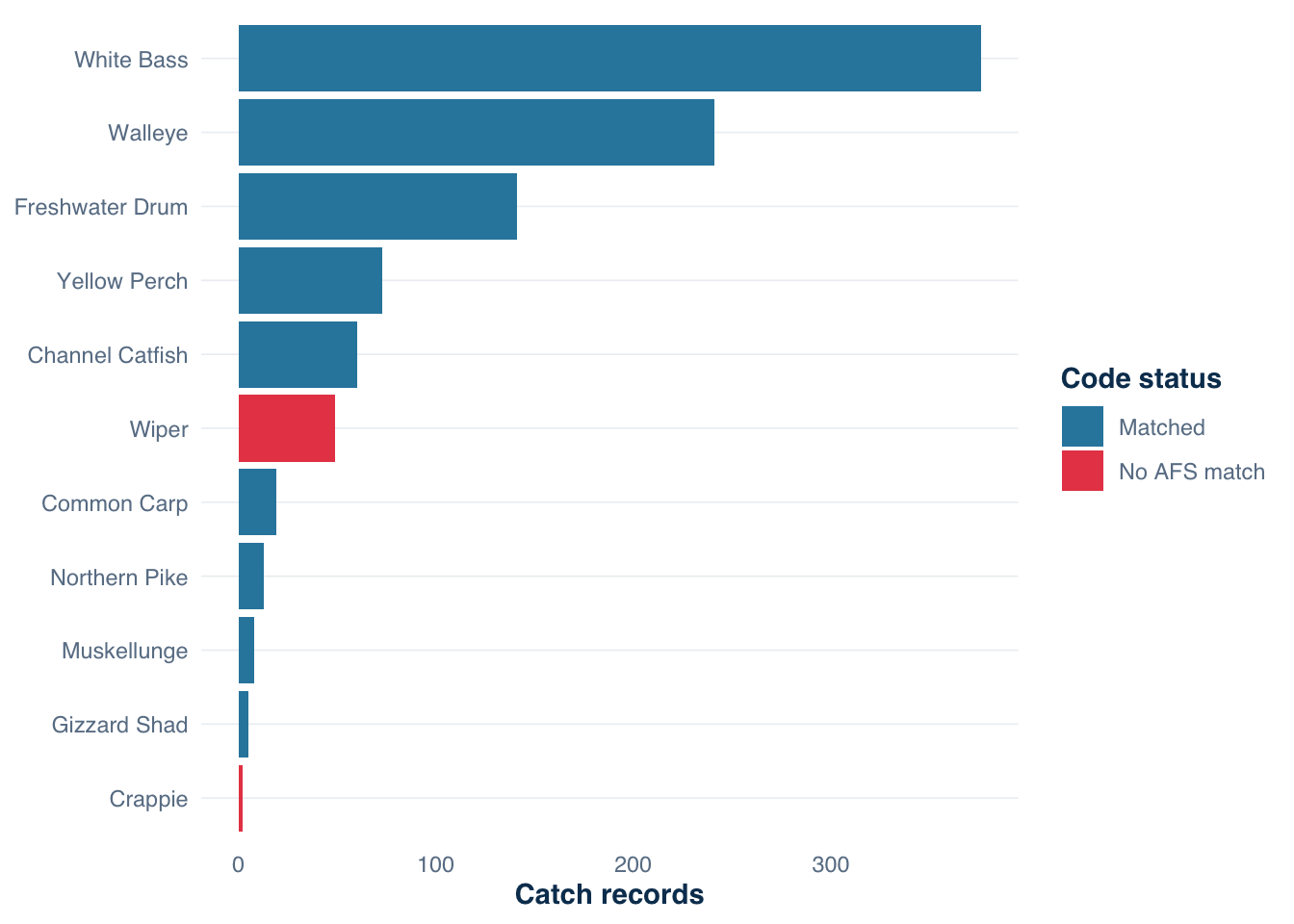
The Harlan catch table contains 11 species entered as free-text common names. Most of these map cleanly to AFS codes:

standardize_species(harlan_catch) |>
  select(species, species_code) |>
  distinct() |>
  arrange(is.na(species_code), species)

Warning: 2 species value(s) could not be matched to an
AFS code and will be "NA":
• "Wiper"
• "Crappie"

# A tibble: 11 × 2
   species         species_code
   <chr>           <chr>       
 1 Channel Catfish CCF         
 2 Common Carp     CRP         
 3 Freshwater Drum FRD         
 4 Gizzard Shad    GPS         
 5 Muskellunge     MUE         
 6 Northern Pike   NOP         
 7 Walleye         WAE         
 8 White Bass      WHB         
 9 Yellow Perch    YEP         
10 Crappie         <NA>        
11 Wiper           <NA>        

Nine of eleven species resolve to AFS codes. Two do not: Wiper and Crappie. (Freshwater Drum, which lacked an AFS code in earlier versions, now resolves automatically to "FRD" in tidycreel ≥ 2.2.0.)

Wiper is a Striped Bass × White Bass hybrid that varies in naming by region and lacks a single-code standard. Crappie entered without species designation is a data quality issue: Black Crappie and White Crappie are distinct management units in many systems, and pooled entries cannot be split after the fact.

These are different problems. Wiper needs a project-specific code assignment. Crappie needs a conversation with field staff about whether species-level identification was attempted and, if so, how to recover it from supplemental records.

Warning: 2 species value(s) could not be matched to an
AFS code and will be "NA":
• "Wiper"
• "Crappie"

Figure 19.1: Species in the Harlan Reservoir 2022 catch records by AFS code match status. Matched species resolve to standard codes and are ready for cross-survey comparison. Unmatched species require manual resolution before merging with external data.

What to do when codes are missing

When standardize_species() returns NA for a species, the analyst has three options, and the choice should be documented:

1. Assign a project code for species that have no universal standard but can be coded consistently (Wiper). Pass a named character vector via the custom_codes argument — standardize_species(data, custom_codes = c("Wiper" = "WPR")) — or apply a case_when() override to the species_code column after the function runs.
2. Create a pooled category for entries that mix species (Crappie without species designation). A project-specific label like "CRP-POOL" flags the record as unresolved without discarding the catch count.
3. Flag as unresolved and exclude from species totals if the entry cannot be reliably coded without returning to field records. Report species totals only for rows where !is.na(species_code).

A case_when() override handles the two remaining unresolved species after standardize_species() runs. For single-species overrides, custom_codes = c("Wiper" = "WPR") is equivalent; case_when() is used here because Crappie requires a pooled label ("CRP-POOL") that warrants explicit documentation in the code:

harlan_catch_coded <- harlan_catch |>
  standardize_species() |>
  mutate(species_code = case_when(
    species == "Wiper"   ~ "WPR",      # project code; no AFS standard
    species == "Crappie" ~ "CRP-POOL", # pooled: species unknown
    TRUE                 ~ species_code
  ))

Warning: 2 species value(s) could not be matched to an
AFS code and will be "NA":
• "Wiper"
• "Crappie"

harlan_catch_coded |>
  select(species, species_code) |>
  distinct() |>
  arrange(is.na(species_code), species)

# A tibble: 11 × 2
   species         species_code
   <chr>           <chr>       
 1 Channel Catfish CCF         
 2 Common Carp     CRP         
 3 Crappie         CRP-POOL    
 4 Freshwater Drum FRD         
 5 Gizzard Shad    GPS         
 6 Muskellunge     MUE         
 7 Northern Pike   NOP         
 8 Walleye         WAE         
 9 White Bass      WHB         
10 Wiper           WPR         
11 Yellow Perch    YEP         

After the override, all 11 species in the Harlan dataset have a code. (Nine resolved automatically via the AFS lookup; two required the case_when() step.) The "CRP-POOL" label is a signal to downstream reporting code that this entry should not be summed with species-level Crappie totals from other sources. Any consistent, documented label works; what matters is that the convention is applied identically in every reporting cycle.

19.3 Referential integrity between tables

A creel dataset is a set of linked tables: a schedule table, an interview table, and a catch table. Cleaning a single table without checking the others can leave the dataset in an inconsistent state. The most common failure modes are:

• Orphan catch records — catch rows whose interview_id does not match any interview. These inflate species totals without contributing effort or trip information.
• Zero-catch interviews — interview rows with no matching catch records. These are usually valid (skunked anglers), but a large count may signal a data entry gap.

A pair of anti_join() calls checks both conditions:

# Catch records with no parent interview
anti_join(harlan_catch, harlan_interviews, by = "interview_id")

# A tibble: 0 × 4
# ℹ 4 variables: interview_id <int>, species <chr>, catch_type <chr>,
#   n_fish <int>

# Interviews with no catch records at all
anti_join(harlan_interviews, harlan_catch, by = "interview_id") |>
  count(trip_status)

# A tibble: 2 × 2
  trip_status     n
  <chr>       <int>
1 complete       56
2 incomplete    102

The Harlan data passes both checks. The 158 interviews with no catch records are not a data gap: 56 are completed trips and 102 are incomplete trips where the angler reported zero fish caught. Zero-catch completed trips are valid observations and must remain in the analysis.

The second check is worth running any time the catch table and interview table arrive from different sources — for example, when interview data is collected in a mobile app and catch data is added later from a separate entry screen. In that workflow, late-arriving catch records that reference deleted interview IDs would appear as orphans here.

When an orphan catch record is found, the response depends on whether the interview can be recovered. If the interview was not entered, the catch record should be removed. If the interview was entered under a different ID (a key mismatch, common in manual entry), the catch record should be relinked. Either way, the decision should be logged.

19.4 Trip duration: plausibility and outlier review

Why hours_fished is sensitive

The hours_fished field is the effort denominator for catch-per-unit-effort estimates. Its mean value among complete trips drives the CPUE calculation directly: CPUE = (total catch) / (total hours fished). An extreme value in hours_fished inflates the denominator, deflates the CPUE, and, if the associated catch is high, distorts both the effort and catch components.

Access-point surveys at Harlan are scheduled in two periods: morning (period 1, 8-hour window) and afternoon/evening (period 2, 6-hour window). A trip duration exceeding the scheduled window for that period is physically impossible if the angler’s entire trip occurred within the survey shift. Durations approaching the shift ceiling are plausible but warrant review.

Identifying outliers with flag_outliers()

flag_outliers() implements Tukey’s IQR fence method. For a numeric column with first quartile Q_1 and third quartile Q_3:

\text{fence\_high} = Q_3 + k \times \text{IQR}

Values above the upper fence are flagged as outliers. The multiplier k controls sensitivity. Tukey’s conventional choices are k = 1.5 for mild outliers and k = 3.0 for extreme outliers.

flag_outliers(harlan_interviews, hours_fished, k = 1.5) |>
  filter(is_outlier) |>
  select(interview_id, date, day_type, period, trip_status,
         hours_fished, fence_high, outlier_reason)

ℹ 1 of 600 values flagged as outliers in hours_fished (k = 1.5, fence:
  [-5.5237, 12.1662]).

# A tibble: 1 × 8
  interview_id date       day_type period trip_status hours_fished fence_high
         <int> <date>     <chr>     <dbl> <chr>              <dbl>      <dbl>
1          388 2022-07-14 weekday       2 complete            13.8       12.2
# ℹ 1 more variable: outlier_reason <chr>

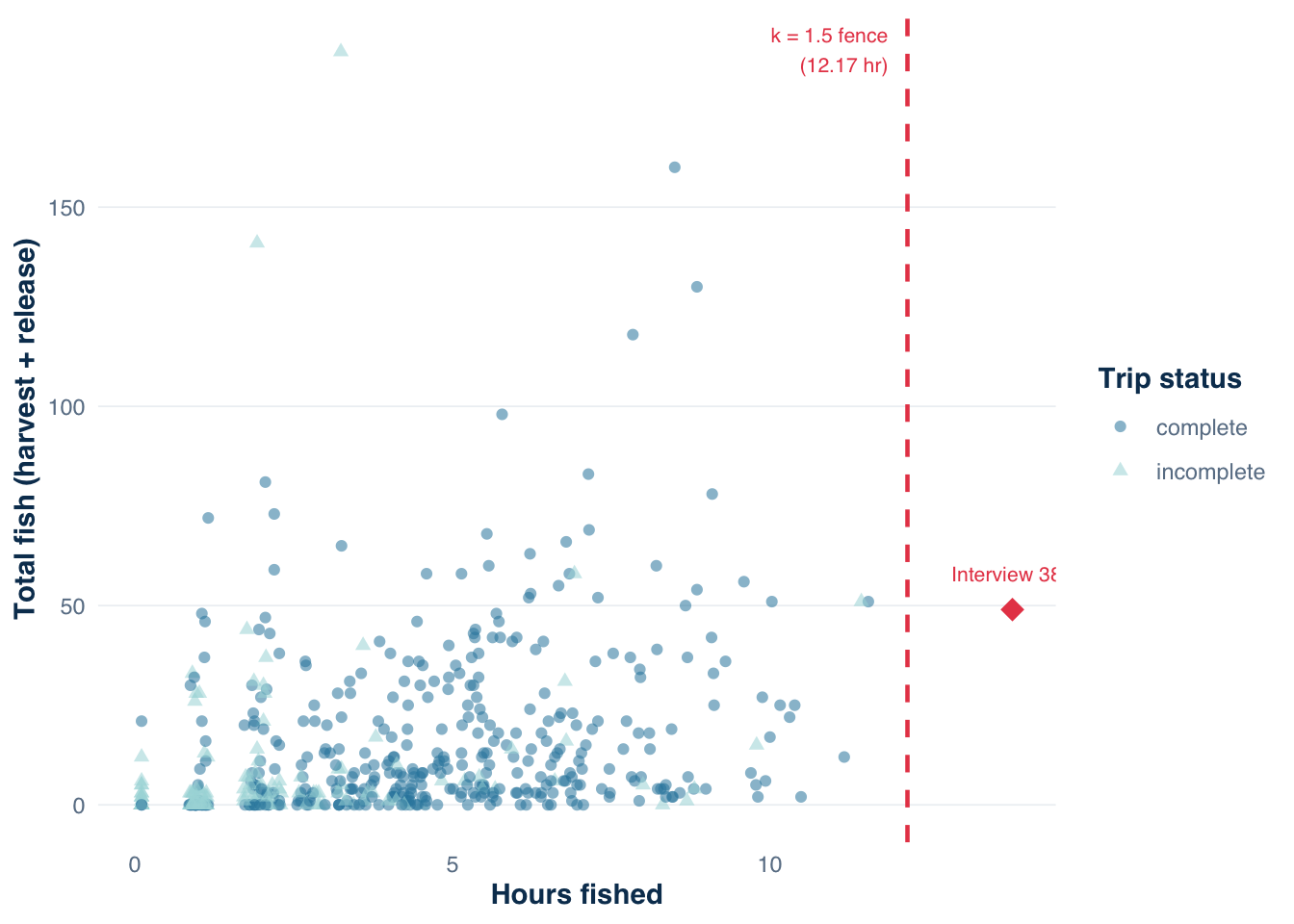
At k = 1.5, one interview is flagged: interview 388, recorded on 14 July 2022, with hours_fished = 13.82. The upper fence at k = 1.5 is Q_3 + 1.5 \times \text{IQR} = 5.53 + 1.5 \times 4.42 = 12.17 hours. Interview 388 exceeds that fence.

flag_outliers(harlan_interviews, hours_fished, k = 3.0) |>
  filter(is_outlier) |>
  select(interview_id, date, day_type, trip_status, hours_fished,
         fence_high, outlier_reason)

ℹ 0 of 600 values flagged as outliers in hours_fished (k = 3, fence: [-12.1575,
  18.8]).

# A tibble: 0 × 7
# ℹ 7 variables: interview_id <int>, date <date>, day_type <chr>,
#   trip_status <chr>, hours_fished <dbl>, fence_high <dbl>,
#   outlier_reason <chr>

At k = 3.0, the upper fence rises to 5.53 + 3.0 \times 4.42 = 18.80 hours. No records are flagged. A 13.82-hour trip falls within the extreme-outlier fence.

The choice between k = 1.5 and k = 3.0 is not mechanical. For a survey with 14-hour interview windows, a 13.82-hour trip is unusual but physically possible. Whether to treat it as an error depends on whether the survey period for that record permitted a trip that long. The right question is not whether the value is statistically unusual but whether it is substantively implausible given the field conditions.

In this case, interview 388 is classified as a completed trip on a weekday in period 2 (the 6-hour window). A completed trip of 13.82 hours in a 6-hour window is impossible — the angler could not have completed a 13.82-hour trip within the survey period if the period only ran 6 hours. That physical constraint justifies flagging and reviewing, regardless of which k value the IQR fence produced.

Visualizing duration against catch

A univariate view of hours_fished shows where the fence falls. A bivariate view — hours fished against total fish caught — reveals whether a flagged record is unusual in one dimension only or in both simultaneously.

ℹ 1 of 600 values flagged as outliers in hours_fished (k = 1.5, fence:
  [-5.5237, 12.1662]).

Figure 19.2: Hours fished versus total fish caught (harvest + release) per interview at Harlan Reservoir 2022. Each point is one interview, colored by trip status. Interview 388 (13.82 hr, 49 fish) sits at the far right — the longest trip in the dataset. The dashed vertical line marks the k = 1.5 IQR outlier fence for hours_fished (12.17 hr). Several other complete trips show high catch counts (up to 189 fish) with shorter durations, indicating that duration and catch quantity are weakly correlated at Harlan.

Interview 388 is the rightmost point: the longest trip in the dataset at 13.82 hours with a moderate catch of 49 fish. It is unusual for its duration, not for its catch count. Trips with far higher catch totals (up to 189 fish) appear throughout the dataset with much shorter durations, demonstrating that hours fished and total catch are only weakly correlated at Harlan. That weak correlation is itself informative: it means no single threshold on either variable alone is sufficient to identify implausible combinations. A trip with low duration and unusually high catch (for example, 189 fish in 1.92 hours, visible in the upper-left region of the plot) deserves the same scrutiny as a trip with unusually long duration.

What to do with flagged duration records

The appropriate response to a flagged trip duration depends on the source of the anomaly:

• Transcription error — if field sheets show a different value, correct to the field record and document the correction.
• Plausible but unusual — if the value is consistent with the field record, retain the record and note in the analysis log that one complete trip exceeded the k = 1.5 fence. No correction is needed.
• Inconsistent with survey design — if the duration is impossible given the survey period (as in the period-2 case above), reclassify the trip as incomplete, truncate hours_fished to the period boundary, or remove the record. Each option changes the estimate differently.

The conservative default is to flag, document, and retain — then report sensitivity to the analyst’s choice (see Section 19.9).

19.5 Catch quantities: large bags and zero-catch trips

Flag_outliers on fish counts

The same IQR fence logic applies to fish counts. Large bag totals can arise from two distinct causes: data entry error (clerk transcribed “32” instead of “2”) or genuine large catch (angler found a schooling White Bass aggregation and limited out on multiple species). The fence identifies which records are statistically unusual; field knowledge determines which are substantively suspicious.

flag_outliers(harlan_catch, n_fish, k = 1.5) |>
  filter(is_outlier) |>
  count(species) |>
  arrange(desc(n))

ℹ 99 of 987 values flagged as outliers in n_fish (k = 1.5, fence: [-11, 21]).

# A tibble: 4 × 2
  species             n
  <chr>           <int>
1 White Bass         64
2 Walleye            30
3 Freshwater Drum     4
4 Yellow Perch        1

At k = 1.5, 99 of 987 catch records exceed the fence at 21 fish. The distribution is dominated by White Bass and Walleye. White Bass at Harlan school aggressively during spring and fall; bag limits in Nebraska permit daily limits that can produce interview-level totals well above 21. Walleye with high counts may reflect multi-angler parties (the n_anglers field records the party, not the individual, at Harlan) or productive early-season trips.

These records are not errors in the conventional sense. They are real, they are high, and they are the result of field conditions that the survey is designed to capture. Removing them would bias harvest estimates downward by systematically excluding high-catch parties.

Zero-catch and zero-effort records

Zero catches are common and valid. An angler who fished all morning and caught nothing represents a real data point: zero catch, positive effort. That zero enters the CPUE denominator appropriately.

What requires attention is zero effort on a completed trip. A record with trip_status == "complete" and hours_fished == 0 is internally inconsistent: a completed trip must have positive effort. The Harlan data contains no such records:

harlan_interviews |>
  filter(hours_fished == 0 | (trip_status == "complete" & hours_fished < 0.1))

# A tibble: 0 × 12
# ℹ 12 variables: reservoir <chr>, date <date>, day_type <chr>, period <dbl>,
#   section <chr>, interview_id <int>, party_id <chr>, n_anglers <dbl>,
#   angler_type <chr>, angler_method <chr>, hours_fished <dbl>,
#   trip_status <chr>

Zero-catch records, on the other hand, are present and expected. Interviews with no associated catch records in harlan_catch represent skunked parties — valid observations that enter the estimator with catch = 0.

Context-dependent review

Flagging catch counts at k = 1.5 casts a wide net. A more defensible approach pairs the flag with domain knowledge:

1. Compare flagged values against legal bag limits for each species. A White Bass count of 32 is plausible (Nebraska has no closed season and a liberal bag limit). A Walleye count of 49 in a single interview warrants a second look at field sheets.
2. Check whether the party size (n_anglers) is large enough to explain the count. An interview with n_anglers = 4 and 32 White Bass is 8 fish per person — straightforward. An interview with n_anglers = 1 and 49 Walleye is 49 individual fish — warranting field record review.

The Harlan catch record with the highest outlier flag is 49 Walleye released by a single party (interview 388 — the same record flagged for unusual trip duration). The combination of an implausible trip duration and an unusually large Walleye release count in the same interview strengthens the case for field record review.

19.6 Party size and angler counts

The n_anglers field records the number of anglers in the interviewed party. At Harlan, parties range from 1 to 9:

harlan_interviews |>
  count(n_anglers) |>
  mutate(pct = round(n / sum(n) * 100, 1))

# A tibble: 9 × 3
  n_anglers     n   pct
      <dbl> <int> <dbl>
1         1   141  23.5
2         2   312  52  
3         3    85  14.2
4         4    45   7.5
5         5     7   1.2
6         6     5   0.8
7         7     1   0.2
8         8     3   0.5
9         9     1   0.2

Most parties are 1–2 anglers (75.5%). Parties of 7–9 exist but are rare (0.9% of interviews). At k = 1.5, flag_outliers() sets the fence at 2 anglers, flagging all parties of 3 or more — nearly half the dataset. This illustrates why k must be calibrated to the variable’s natural distribution: n_anglers is right-skewed but parties of 3 or more are not errors. For discrete count variables with low expected maxima, domain-specific absolute bounds are more useful than IQR fences.

At Harlan, a reasonable absolute upper bound is 8 anglers per interview — a figure consistent with a typical boat capacity plus family bank fishing. A single record exceeds that bound:

harlan_interviews |>
  filter(n_anglers > 8) |>
  select(interview_id, date, angler_type, n_anglers, hours_fished, trip_status)

# A tibble: 1 × 6
  interview_id date       angler_type n_anglers hours_fished trip_status
         <int> <date>     <chr>           <dbl>        <dbl> <chr>      
1          273 2022-05-26 boat                9         6.95 complete   

Interview 273 recorded 9 anglers on a weekday in May. Nine anglers is physically plausible for a group outing but worth confirming against the field sheet — both because party size affects the angler-effort denominator and because the interview represents 9 angler-trips in the catch rate calculation. One misrecorded party of 9 that should have been 2 would contribute 4.5× the weight it deserves.

A more reliable check is joint consistency between party size and catch. A party of 2 anglers reporting 6 Walleye harvested is plausible. A party of 2 reporting 90 Walleye harvested is not. That joint check requires pairing the interview table with the catch table:

harlan_interviews |>
  left_join(
    harlan_catch |>
      filter(catch_type == "harvested") |>
      group_by(interview_id) |>
      summarise(total_harvest = sum(n_fish), .groups = "drop"),
    by = "interview_id"
  ) |>
  mutate(
    total_harvest      = replace_na(total_harvest, 0),
    harvest_per_angler = total_harvest / n_anglers
  ) |>
  filter(harvest_per_angler > 15) |>
  select(interview_id, date, n_anglers, total_harvest, harvest_per_angler,
         trip_status, hours_fished)

# A tibble: 8 × 7
  interview_id date       n_anglers total_harvest harvest_per_angler trip_status
         <int> <date>         <dbl>         <int>              <dbl> <chr>      
1           20 2022-09-08         2            35               17.5 complete   
2           57 2022-09-23         1            17               17   complete   
3           59 2022-06-08         2            34               17   complete   
4          520 2022-05-13         2            31               15.5 incomplete 
5          528 2022-05-15         1            17               17   complete   
6          539 2022-05-16         4            62               15.5 complete   
7          557 2022-05-20         2            32               16   complete   
8          562 2022-05-22         1            17               17   complete   
# ℹ 1 more variable: hours_fished <dbl>

Any interview with more than 15 harvested fish per angler — a threshold that exceeds legal bag limits for most target species in this system — surfaces as a candidate for field record review.

19.7 Trip status as a cleaning variable

Trip status (complete versus incomplete) is not just a classification field. It determines which records enter which estimator:

• Complete trips contribute to CPUE estimation (ratio-of-means uses completed trips only; see Section 20.3 and Section 22.2).
• Incomplete trips are used by some estimators to validate that complete and incomplete anglers are exchangeable (see validate_incomplete_trips() in Section 10.9).

A misclassified trip status is therefore a cleaning decision with a direct pathway into the estimate. An incomplete trip recorded as complete inflates the hours-fished denominator of CPUE (incomplete trips are shorter on average). A complete trip recorded as incomplete removes a valid observation from the ratio estimator.

The Harlan data shows the expected pattern: complete trips are longer than incomplete trips, with little overlap in their medians:

summarize_trips(harlan_design_ch11)

Trip Status Summary

Total interviews: 600
  Complete:   390 (65%)
  Incomplete: 210 (35%)

Duration (hours) by status:
  complete: min=0.1, median=4.55, mean=4.74, max=13.82
  incomplete: min=0.1, median=1.06, mean=1.71, max=11.44

The complete trip mean is 4.74 hours; the incomplete trip mean is 1.71 hours. The ratio (2.77) is consistent with access-point survey literature where incomplete trips typically represent early-arriving anglers intercepted before they finish. If those means were reversed — or if incomplete trip durations clustered near the shift ceiling — misclassification would be a prime suspect.

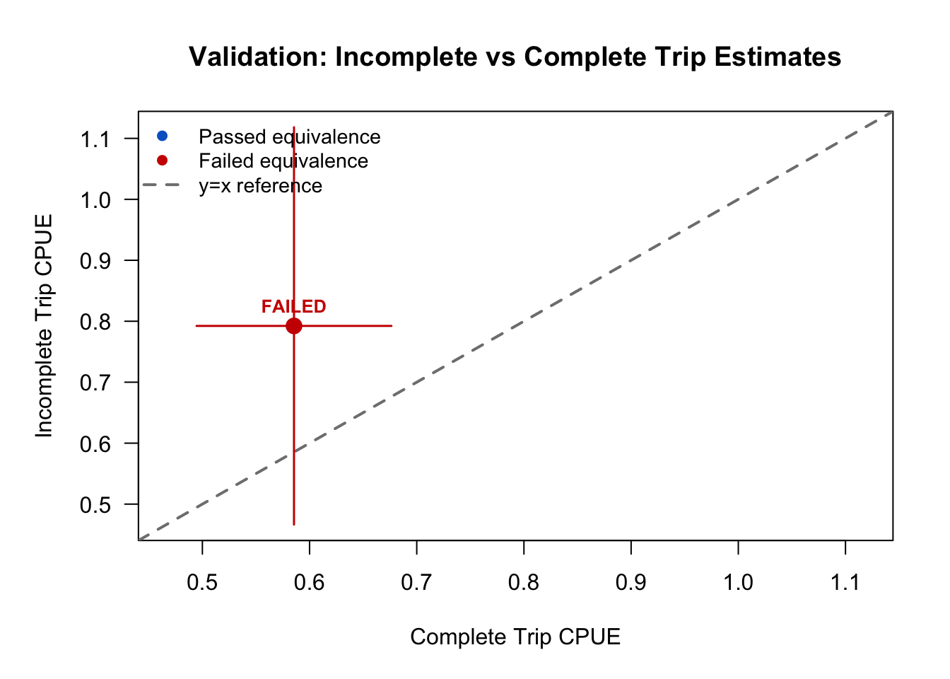
validate_incomplete_trips() tests whether the two groups are statistically exchangeable for catch-rate estimation using two one-sided tests (TOST) within a specified equivalence margin:

validate_incomplete_trips(
  harlan_design_ch11,
  catch      = total_harvest,
  effort     = hours_fished,
  truncate_at = 0.5
)

── TOST Equivalence Validation Results ─────────────────────────────────────────
Threshold: ±20% of complete trip estimate
✖ Validation FAILED

Recommendation: Validation failed: Use complete trips only (estimates not
statistically equivalent)


── Overall Test ──

Complete trips: n = 390, CPUE = 0.585
Incomplete trips: n = 152, CPUE = 0.792
Difference: -0.207
Equivalence bounds: [-0.117, 0.117]
TOST p-values: p_lower = 0.6981, p_upper = 0.0313
✖ Overall equivalence: FAILED

The test fails. Incomplete trips at Harlan catch at a meaningfully higher rate than complete trips (0.792 vs. 0.585 fish/hr), and the difference falls outside the ±20% equivalence margin. The TOST failure does not indicate that trip status was misclassified — it indicates that incomplete anglers systematically differ from complete anglers, a common pattern at access-point surveys where early- morning arrivals target faster-biting periods. Keep the groups separate. Any record misclassified as “complete” that truly represents a shorter, higher-intensity trip would inflate the complete-trip catch rate and bias CPUE estimates upward.

19.8 Building a cleaning log

Any cleaning step that changes a record’s contribution to an estimate should be logged before it is applied. A minimal cleaning log has four columns per changed record: the record identifier, the field affected, the original value, and the new value. A fifth column should capture the rule applied.

The dplyr approach keeps the raw data intact and stores changes as a separate audit table:

cleaning_log <- harlan_interviews |>
  left_join(
    flag_outliers(harlan_interviews, hours_fished, k = 1.5) |>
      select(interview_id, is_outlier, fence_high),
    by = "interview_id"
  ) |>
  filter(is_outlier) |>
  mutate(
    field         = "hours_fished",
    original_value = hours_fished,
    proposed_value = fence_high,
    rule           = "IQR k=1.5: hours_fished exceeds upper fence; review against field record",
    action         = "REVIEW — do not apply automatically"
  ) |>
  select(interview_id, date, day_type, period, trip_status,
         field, original_value, proposed_value, rule, action)

ℹ 1 of 600 values flagged as outliers in hours_fished (k = 1.5, fence:
  [-5.5237, 12.1662]).

cleaning_log

# A tibble: 1 × 10
  interview_id date       day_type period trip_status field       original_value
         <int> <date>     <chr>     <dbl> <chr>       <chr>                <dbl>
1          388 2022-07-14 weekday       2 complete    hours_fish…           13.8
# ℹ 3 more variables: proposed_value <dbl>, rule <chr>, action <chr>

The key discipline is the action column. A cleaning log is not a deletion list. It is a record of anomalies and proposed responses. The final decision — accept, correct, or remove — should be recorded before the analysis runs, not reconstructed after the fact.

For the one flagged duration record (interview 388), the proposed action is field record review. Until that review is complete, the defensible choice is to run the analysis twice: once with the record retained and once with it excluded, and report the sensitivity.

Applying a cleaning decision in code

Once a cleaning decision is made, the implementation follows one of three patterns depending on the action taken. All three keep the raw data unchanged and produce a derived cleaned dataset:

# Option 1: truncate hours_fished to the period boundary (6 hr for period 2)
interviews_truncated <- harlan_interviews |>
  mutate(
    hours_fished = case_when(
      interview_id == 388 ~ 6.0,   # period 2 maximum
      TRUE                ~ hours_fished
    )
  )

# Option 2: remove the record entirely
interviews_removed <- harlan_interviews |>
  filter(interview_id != 388)

# Option 3: reclassify trip status to incomplete (then drop from CPUE)
interviews_reclassified <- harlan_interviews |>
  mutate(
    trip_status = if_else(interview_id == 388, "incomplete", trip_status)
  )

# Show effect on mean complete trip duration
list(
  original      = harlan_interviews,
  truncated     = interviews_truncated,
  removed       = interviews_removed,
  reclassified  = interviews_reclassified
) |>
  map_dfr(
    ~ filter(.x, trip_status == "complete") |>
        summarise(n = n(), mean_hr = mean(hours_fished), max_hr = max(hours_fished)),
    .id = "approach"
  )

# A tibble: 4 × 4
  approach         n mean_hr max_hr
  <chr>        <int>   <dbl>  <dbl>
1 original       390    4.74   13.8
2 truncated      390    4.72   11.6
3 removed        389    4.72   11.6
4 reclassified   389    4.72   11.6

Each option shifts the mean complete trip duration by a different amount. Truncation to 6.0 hours reduces the mean most aggressively because 6.0 is well below interview 388’s recorded value. Removal reduces it more modestly because it eliminates one observation. Reclassification to incomplete removes the record from the complete-trip pool entirely, producing the same result as removal for CPUE estimation. Which option matches the field record determines which is correct — not statistical convenience.

19.9 The estimation impact

How a single record propagates

Interview 388 (13.82 hours, complete, 49 Walleye released, 0 harvested) enters the analysis in two places: the trip duration distribution used to compute mean hours_fished among complete trips, and the catch table as 49 released Walleye. Removing it produces two changes:

Trip duration summary — the mean complete trip duration shifts from 4.74 to 4.72 hours (removing 0.02 hours from the mean of 390 complete trips):

# Design without interview 388
design_clean <- build_design(
  filter(harlan_interviews_with_catch, interview_id != 388),
  filter(harlan_catch, interview_id != 388)
)

# Compare trip summaries
cat("--- Full dataset ---\n")

--- Full dataset ---

summarize_trips(harlan_design_ch11)

Trip Status Summary

Total interviews: 600
  Complete:   390 (65%)
  Incomplete: 210 (35%)

Duration (hours) by status:
  complete: min=0.1, median=4.55, mean=4.74, max=13.82
  incomplete: min=0.1, median=1.06, mean=1.71, max=11.44

cat("\n--- Interview 388 removed ---\n")

--- Interview 388 removed ---

summarize_trips(design_clean)

Trip Status Summary

Total interviews: 599
  Complete:   389 (64.9%)
  Incomplete: 210 (35.1%)

Duration (hours) by status:
  complete: min=0.1, median=4.53, mean=4.72, max=11.55
  incomplete: min=0.1, median=1.06, mean=1.71, max=11.44

Catch rate (CPUE) — removing the 13.82-hour zero-harvest trip reduces the hours-fished denominator slightly, and CPUE rises from 0.585 to 0.589 fish/hr:

cpue_full  <- estimate_catch_rate(harlan_design_ch11)$estimates

ℹ Using complete trips for CPUE estimation
  (n=390, 65% of 600 interviews) [default]

cpue_clean <- estimate_catch_rate(design_clean)$estimates

ℹ Using complete trips for CPUE estimation
  (n=389, 64.9% of 599 interviews) [default]

bind_rows(
  cpue_full  |> mutate(dataset = "Full (n = 390 complete trips)"),
  cpue_clean |> mutate(dataset = "Interview 388 removed (n = 389)")
) |>
  select(dataset, estimate, se, ci_lower, ci_upper, n)

# A tibble: 2 × 6
  dataset                         estimate     se ci_lower ci_upper     n
  <chr>                              <dbl>  <dbl>    <dbl>    <dbl> <int>
1 Full (n = 390 complete trips)      0.585 0.0464    0.495    0.676   390
2 Interview 388 removed (n = 389)    0.589 0.0466    0.498    0.681   389

The absolute difference is 0.004 fish/hr — small relative to the 95% confidence interval width of 0.18 fish/hr. In this case, retaining or removing interview 388 does not materially change the conclusion. That result should be reported explicitly: “Sensitivity analysis: removing the one trip duration outlier changed the CPUE estimate by 0.004 fish/hr (0.7%), within the uncertainty of the estimate.”

What if the catch classification were wrong?

The CPUE analysis above tests the impact of removing a record. A different class of cleaning error — a catch-type misclassification — has a different propagation path. Consider the question: what if interview 388 had the 49 Walleye entered as harvested rather than released, and the misclassification went undetected?

That scenario does not change the hours-fished denominator. It does change the harvest numerator. The effect is isolated to estimate_total_harvest():

# Hypothetical: 49 released Walleye entered as harvested (catch_type error)
catch_whatif <- harlan_catch |>
  mutate(
    catch_type = if_else(
      interview_id == 388 & species == "Walleye",
      "harvested",
      catch_type
    )
  )

design_whatif <- build_design_harvest(catch_whatif)

bind_rows(
  estimate_total_harvest(harlan_design_ch11_harvest)$estimates |>
    mutate(scenario = "Actual (49 Walleye released)"),
  estimate_total_harvest(design_whatif)$estimates |>
    mutate(scenario = "What-if (49 Walleye entered as harvested)")
) |>
  select(scenario, estimate, se, ci_lower, ci_upper)

# A tibble: 2 × 5
  scenario                                  estimate    se ci_lower ci_upper
  <chr>                                        <dbl> <dbl>    <dbl>    <dbl>
1 Actual (49 Walleye released)                11052. 1507.    8092.   14012.
2 What-if (49 Walleye entered as harvested)   11228. 1529.    8226.   14231.

Reclassifying 49 released Walleye as harvested in one interview adds approximately 177 fish to the season harvest estimate — a 1.6% upward bias. The reason the expansion factor is roughly 3.6× (not 1.0×) is that the stratified estimator treats this interview’s harvest rate as representative of other complete trips in the same stratum. One high-catch record inflates the stratum-level mean, which then multiplies against the total estimated effort.

Whether 177 fish is material depends on the management context. For a fishery with a Walleye quota or a slot-limit assessment, a 1.6% harvest overestimate matters. For a general community harvest summary, it may be within acceptable reporting uncertainty. The point is not the magnitude in isolation. The analyst should compute it and make the judgment explicitly rather than assume catch-type errors are harmless.

When the impact is not small

The Harlan example is clean enough that one outlier has minimal effect. In programs with smaller sample sizes (50–80 interviews per stratum), a single anomalous record can move a CPUE estimate by 5–10%. The same analysis — run twice, compare the difference — is still the right approach. The magnitude of the sensitivity result determines whether the record requires resolution before the report is finalized.

A cleaning decision that shifts the estimate by more than the reported uncertainty (i.e., by more than the half-width of the confidence interval) is a decision that should be documented in the methods section, not buried in a data appendix.

Effort estimates are less sensitive

The total effort estimate (angler-hours) comes from instantaneous count expansion, not from hours_fished in the interview table. Removing interview 388 does not change the count-based effort estimate:

bind_rows(
  estimate_effort(harlan_design_ch11, target = "stratum_total")$estimates |>
    mutate(dataset = "Full"),
  estimate_effort(design_clean, target = "stratum_total")$estimates |>
    mutate(dataset = "Interview 388 removed")
) |>
  select(dataset, estimate, se, ci_lower, ci_upper)

Warning: Count variable angler_hours contains 18 zero values.
ℹ Zero values may indicate days with no fishing activity or data collection
  issues.
ℹ Consider whether zeros are true zeros or missing data.
Count variable angler_hours contains 18 zero values.
ℹ Zero values may indicate days with no fishing activity or data collection
  issues.
ℹ Consider whether zeros are true zeros or missing data.

# A tibble: 2 × 5
  dataset               estimate    se ci_lower ci_upper
  <chr>                    <dbl> <dbl>    <dbl>    <dbl>
1 Full                    33052. 3704.   25716.   40388.
2 Interview 388 removed   33052. 3704.   25716.   40388.

Both designs produce the same 33,052 angler-hour estimate. This illustrates an important structural feature of the access-point estimator: effort comes from counts, not from interviews. Cleaning decisions that affect the interview table propagate into catch-rate estimates (CPUE, total harvest) but not into the count-based effort expansion. The two components should be diagnosed separately.

19.10 A conservative cleaning rule

The practical guidance from this chapter reduces to four steps:

1. Flag before removing. Use flag_outliers() and standardize_species() to identify anomalies. Do not delete records at the flagging step.

2. Return to field records for flagged entries. A statistical flag is a referral, not a verdict. Check the original data sheet before altering any value.

3. Log every change. Keep the original value, the corrected value, the rule applied, and the interview ID in a cleaning log that travels with the analysis.

4. Report sensitivity. Run the analysis with and without each cleaning decision that materially affects an estimate. If the difference is within the confidence interval, say so. If it is not, the decision requires explicit justification in the methods section.

These steps are not additional overhead. They are the documentation that makes an estimate reproducible — by the same analyst next season, by a reviewer, or by a manager who needs to understand why this year’s estimate differs from last year’s.

19.11 Takeaway

Data cleaning in creel surveys is part of estimation. Decisions about which records to accept, recode, or remove propagate through catch rates, harvest totals, and the uncertainty reported around them. The species name an angler gives in the field, the trip duration a clerk records, and the catch count that enters the database are all measurements, and they benefit from systematic review before being embedded in an estimate.

tidycreel provides flag_outliers() for detecting unusual numeric values and standardize_species() for aligning species names to a common code system. Neither function makes the decision for the analyst. Both functions make the anomalies visible, document the detection rule, and create a foundation for the cleaning log that should accompany every creel analysis.

The Harlan 2022 data required minimal cleaning. One trip duration flagged at k = 1.5; three species names lacked AFS codes; no zero-effort completed trips; no impossible catch counts given the party sizes observed. Those results matter too: a dataset that passes systematic review gives the analyst confidence that the estimates reflect the fishery, not the data entry process.