Code
estimate_catch_rate(harlan_design_ch14)$methodℹ Using complete trips for CPUE estimation
(n=390, 65% of 600 interviews) [default][1] "ratio-of-means-cpue"creel survey, fisheries, design-based inference, R, tidycreel, Quarto
Catch-per-unit-effort (CPUE) compresses the fishing experience into a single ratio: catch divided by effort. That compression is both its appeal and its main source of misinterpretation.
In a roving or access-point creel survey, effort is measured in angler-hours — the product of the number of anglers and the hours they fished. Catch is the number of fish contacted over that same duration. The resulting ratio, in units of fish per angler-hour, is a population-average catch rate: how many fish a representative angler would encounter per hour under the survey conditions.
CPUE is not an index of abundance in the strict sense. A higher CPUE could reflect better fishing conditions, a change in effort distribution, or an actual increase in fish density. It should be labeled as the rate observed under the sampling design, not as a direct measure of population size.
Within a single survey period, however, CPUE is exactly what management reporting requires: an estimate of how productive the fishery appeared to anglers who participated. That quantity, with its uncertainty, is what tidycreel computes from interview records.
There are two ways to form a ratio from interview data, and they answer subtly different questions (Hoenig et al. 1997).
The ratio-of-means (ROM) estimator sums catch and effort separately across all interviews, then divides:
\widehat{\text{CPUE}}_{\text{ROM}} = \frac{\sum_{i=1}^{n} c_i}{\sum_{i=1}^{n} e_i}
where c_i is the total catch for interview i and e_i is the hours fished. This estimator is weighted by trip length: anglers who fished longer contribute more to both the numerator and the denominator. It is the natural estimator for completed trips because the full trip record — final catch and full elapsed hours — is available at the time of interview.
The mean-of-ratios (MOR) estimator computes a per-trip rate for each interview first, then averages those rates:
\widehat{\text{CPUE}}_{\text{MOR}} = \frac{1}{n} \sum_{i=1}^{n} \frac{c_i}{e_i}
This gives each trip equal weight regardless of duration. It is the natural estimator for incomplete trips, where the interview catches an angler mid-trip and c_i and e_i are snapshots of a fishing session still in progress. If the catch process is stationary — if the rate of catching fish does not change systematically within a trip — then the MOR applied to incomplete trips should estimate the same parameter as the ROM applied to completed trips.
The stationarity assumption is the critical qualifier. If anglers learn during a trip, early-trip snapshots will underestimate the completed-trip rate. Hoenig et al. (1997) showed that truncating very short trips reduces bias. The estimator = "mortr" option in estimate_catch_rate() applies this truncation automatically.
Pollock et al. (1994) recommended using completed trips wherever possible because the ROM estimator requires no stationarity assumption, and this book follows that convention wherever the design allows it.
estimate_catch_rate() picks an estimator for you when you do not name one, and which one it picks depends on interview_type, set when the interviews were attached:
interview_type |
use_trips unspecified |
estimator |
|---|---|---|
"access" |
complete trips | ratio-of-means |
"roving" |
all trips | mean-of-ratios |
An access-point design intercepts anglers as they leave, so nearly every record is a finished trip and the ROM is what Pollock et al. (1994) recommends.
Roving is the harder case. The clerk meets anglers mid-trip, so most records are incomplete, and keeping only the complete ones does more than shrink the sample: the trips that happen to be finished when a roving clerk arrives are the long ones, so the surviving subset is biased toward anglers who fish longest. The MOR estimator Hoenig et al. (1997) derived treats each mid-trip contact as its own rate observation and keeps them all, which is why the roving design gets it.
Naming either use_trips or estimator suppresses the selection. The method field reports which estimator ran, so the routing is always checkable. Harlan is access-point, so it reports the ROM:
estimate_catch_rate(harlan_design_ch14)$methodℹ Using complete trips for CPUE estimation
(n=390, 65% of 600 interviews) [default][1] "ratio-of-means-cpue"“Leave it at the default” and “use complete trips” are therefore the same instruction only on an access-point design. On Cedar Lake (Chapter 29), which is roving, the routed harvest rate is 0.81 fish per angler-hour over all 479 contacts; restricting it to complete trips gives 0.76 over 143 — figures from the Cedar chapter, not from the Harlan call above.
The complete-trip rate is the lower of the two, which is the direction Section 9.10 documents at Harlan and for the same reason: anglers who limit out early leave before a clerk can record a finished trip, so the short, high-catch sessions sit in the incomplete pile and the complete-trip subset under-represents them. Length bias and catch-rate bias pull together here rather than cancelling.
Same data, different question, and nothing in the call signature tells you which one you asked. If you mean complete trips, say so.
A practical diagnostic compares both estimators on the same dataset. If the completed and incomplete estimates are close, the stationarity assumption is supported.
The 2022 Harlan Reservoir creel survey collected 600 party interviews. Of those, 390 were completed trips (65%) and 210 were incomplete (35%). The ratio-of-means estimator uses the 390 completed-trip records.
cpue_overall <- estimate_catch_rate(harlan_design_ch14)ℹ Using complete trips for CPUE estimation
(n=390, 65% of 600 interviews) [default]cpue_overall
── Creel Survey Estimates ──────────────────────────────────────────────────────
Method: Ratio-of-Means CPUE
Variance: Taylor linearization
Confidence level: 95%
Unit: fish/angler-hour

# A tibble: 1 × 5
  estimate     se ci_lower ci_upper     n
     <dbl>  <dbl>    <dbl>    <dbl> <int>
1     1.51 0.0928     1.32     1.69   390
The output tibble has five columns: estimate is the ratio-of-means CPUE, se is the Taylor-linearized standard error, ci_lower and ci_upper are the 95% confidence interval bounds, and n is the number of completed-trip interviews.
The overall CPUE estimate is 1.51 fish per angler-hour (95% CI: [1.32, 1.69]). The standard error of 0.093 yields a CV of about 6.2%, which falls comfortably below the 15% precision threshold used in Section 25.1. The 390 completed-trip sample is adequate for a precise ratio estimate at the survey-wide level.
This estimate is the average catch rate for all anglers in all strata combined. It answers the question: how many fish did a typical angler at Harlan encounter per hour in 2022? It does not describe abundance or year-to-year change.
The survey design stratifies the calendar into weekdays and weekends. Weekend days attract different angler populations and can have different crowding, access patterns, and fishing conditions than weekdays. Stratum-specific CPUE separates those effects.
cpue_dt <- estimate_catch_rate(harlan_design_ch14, by = day_type)ℹ Using complete trips for CPUE estimation
(n=390, 65% of 600 interviews) [default]cpue_dt$estimates# A tibble: 2 × 6
day_type estimate se ci_lower ci_upper n
<chr> <dbl> <dbl> <dbl> <dbl> <int>
1 weekday 1.48 0.102 1.28 1.68 321
2 weekend 1.64 0.223 1.21 2.08 69cpue_dt$estimates |>
mutate(
day_type = str_to_title(day_type),
label = sprintf("%.2f (n = %d)", estimate, n)
) |>
ggplot(aes(x = estimate, y = day_type)) +
geom_vline(xintercept = 1.51, linetype = "dashed", colour = "grey50") +
geom_errorbarh(aes(xmin = ci_lower, xmax = ci_upper),
height = 0.15, linewidth = 0.8) +
geom_point(size = 3) +
geom_text(aes(label = label), vjust = -0.8, size = 3.5) +
labs(
x = "CPUE (fish per angler-hour)",
y = NULL,
title = "CPUE by day-type stratum",
caption = "Dashed line: overall estimate (1.51 fish/hr). Error bars: 95% CI."
) +
xlim(0.9, 2.4) +
theme_minimal()Warning: `geom_errorbarh()` was deprecated in ggplot2 4.0.0.
ℹ Please use the `orientation` argument of `geom_errorbar()` instead.`height` was translated to `width`.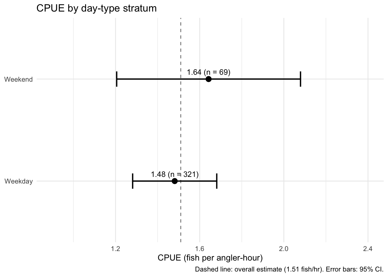
Weekend CPUE (1.64 fish/hr) is slightly higher than weekday CPUE (1.48 fish/hr), but the weekend estimate carries a much wider confidence interval because only 69 weekend interviews were completed trips, compared to 321 weekday interviews.
The interviews distinguish bank anglers from boat anglers. These two groups fish differently: boat anglers can move to productive structure, cover more water, and access mid-lake habitat; bank anglers are constrained to the shoreline. If the fish community or the productive habitat is distributed unevenly, the two groups should show different catch rates.
cpue_at <- estimate_catch_rate(harlan_design_ch14, by = angler_type)ℹ Using complete trips for CPUE estimation
(n=390, 65% of 600 interviews) [default]cpue_at$estimates# A tibble: 2 × 6
angler_type estimate se ci_lower ci_upper n
<chr> <dbl> <dbl> <dbl> <dbl> <int>
1 bank 2.95 0.571 1.83 4.07 71
2 boat 1.41 0.0906 1.23 1.59 319cpue_at$estimates |>
mutate(
angler_type = str_to_title(angler_type),
label = sprintf("%.2f (n = %d)", estimate, n)
) |>
ggplot(aes(x = estimate, y = angler_type)) +
geom_vline(xintercept = 1.51, linetype = "dashed", colour = "grey50") +
geom_errorbarh(aes(xmin = ci_lower, xmax = ci_upper),
height = 0.15, linewidth = 0.8) +
geom_point(size = 3) +
geom_text(aes(label = label), vjust = -0.8, size = 3.5) +
labs(
x = "CPUE (fish per angler-hour)",
y = NULL,
title = "CPUE by angler type",
caption = "Dashed line: overall estimate (1.51 fish/hr). Error bars: 95% CI."
) +
xlim(0, 5) +
theme_minimal()`height` was translated to `width`.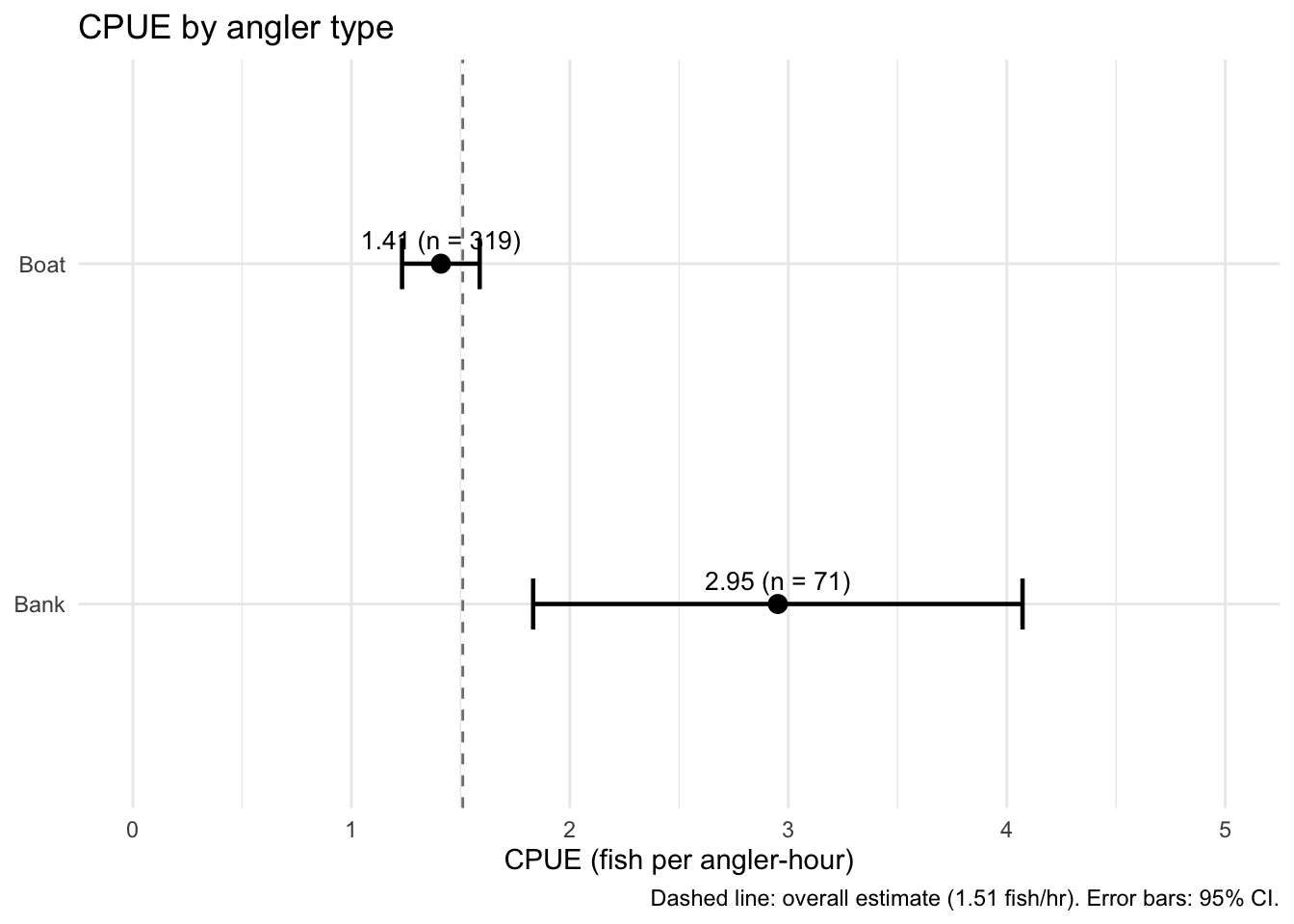
Bank anglers report 2.95 fish per angler-hour (95% CI: [1.83, 4.07]), more than twice the boat angler rate of 1.41 fish/hr (95% CI: [1.23, 1.59]). The comparison still conflates method, location, and target species, so it should not be read as a pure productivity effect.
The choice between ROM and MOR matters most when the dataset contains many incomplete trips and when the analyst suspects non-stationary catch processes. tidycreel provides a diagnostic mode that applies both estimators and compares the results.
cpue_diag <- estimate_catch_rate(harlan_design_ch14, use_trips = "diagnostic")ℹ Running diagnostic comparison
Complete trips (n=390) vs Incomplete trips (n=210)
ℹ Using complete trips for CPUE estimation
(n=390, 65% of 600 interviews)
ℹ Using incomplete trips for CPUE estimation
(n=210, 35% of 600 interviews)cpue_diag$comparison trip_type estimate se ci_lower ci_upper n
1 complete 1.505208 0.0928369 1.323251 1.687165 390
2 incomplete 1.478371 0.2431211 1.001862 1.954880 152The completed-trip estimate is 1.51 fish/hr; the incomplete-trip truncated MOR estimate is 1.48 fish/hr. The difference is 0.027 — less than 2% of the completed-trip value.
The MOR estimate uses 152 of the 210 incomplete-trip interviews; 58 were truncated because the angler had fished fewer than 30 minutes when contacted. Those very short-trip interviews are dropped to avoid leveraging noisy per-trip ratios from anglers who had barely started fishing.
The agreement between estimators for Harlan 2022 suggests that the catch process at Harlan is approximately stationary. This supports using the completed-trip ROM estimate as the primary result.
cpue_diag$comparison |>
  mutate(
    trip_type = str_to_title(trip_type),
    label     = sprintf("%.2f (n = %d)", estimate, n)
  ) |>
  ggplot(aes(x = estimate, y = trip_type)) +
  geom_vline(xintercept = 1.51, linetype = "dashed", colour = "grey50") +
  geom_errorbarh(aes(xmin = ci_lower, xmax = ci_upper),
                 height = 0.15, linewidth = 0.8) +
  geom_point(size = 3) +
  geom_text(aes(label = label), vjust = -0.8, size = 3.5) +
  labs(
    x = "CPUE (fish per angler-hour)",
    y = "Trip type",
    title = "Complete vs incomplete trip CPUE",
    caption = "Dashed line: complete-trip estimate (1.51 fish/hr). Error bars: 95% CI."
  ) +
  xlim(0.5, 2.5) +
  theme_minimal()
`height` was translated to `width`.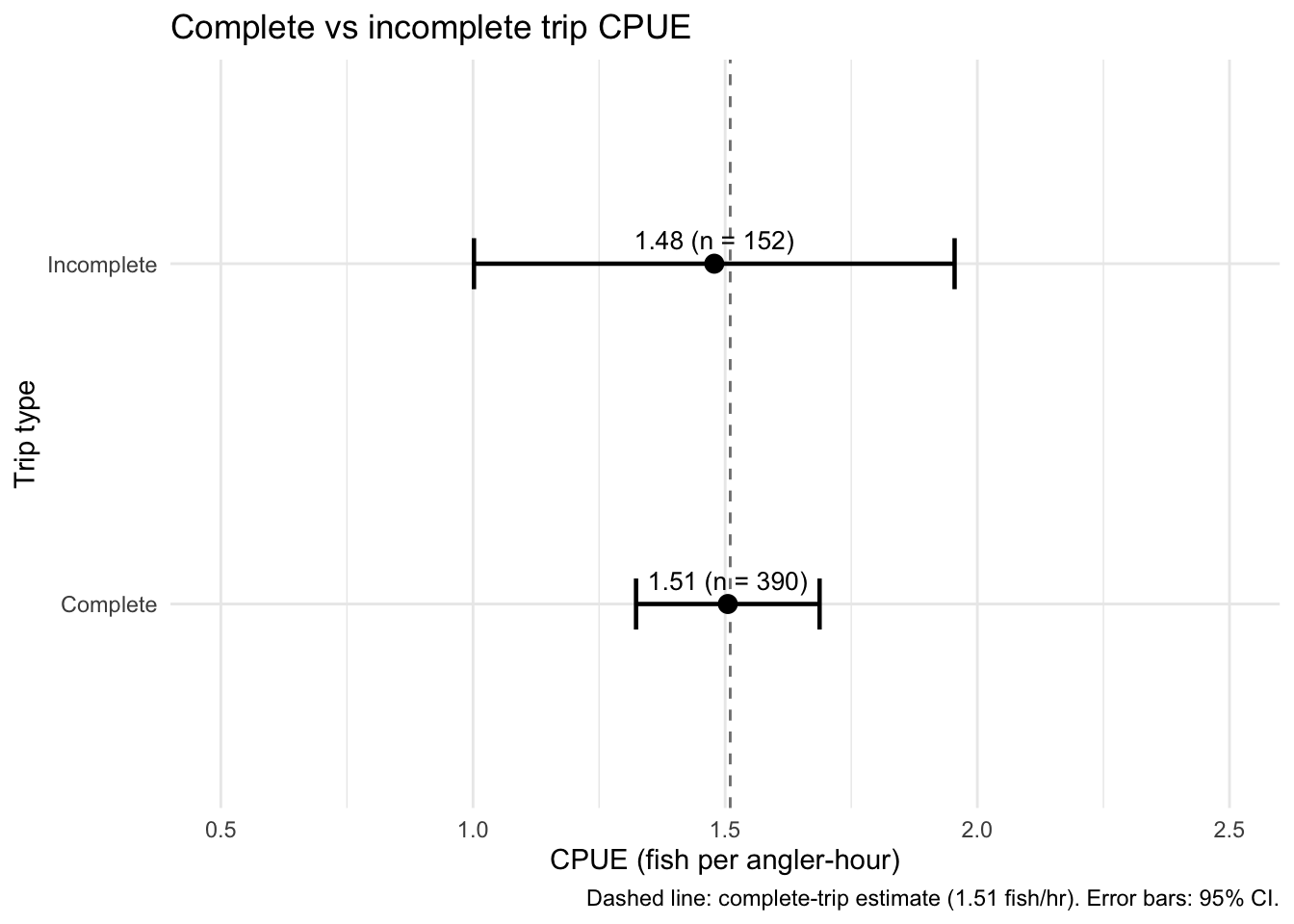
The diagnostic is especially important when the complete-trip sample is small. At Harlan, with 65% complete trips, the diagnostic is confirmatory rather than prescriptive.
CPUE encompasses all fish contacted — harvested and released together. The component rates are estimated separately by estimate_harvest_rate() and estimate_release_rate(). By default these functions also use completed-trip interviews, matching estimate_catch_rate() so that HPUE + RPUE = CPUE exactly.
hpue <- estimate_harvest_rate(harlan_design_ch14)ℹ Filtering to complete trips for HPUE estimation
(n=390, 65% of 600 interviews) [default]rpue <- estimate_release_rate(harlan_design_ch14)ℹ Filtering to complete trips for RPUE estimation
(n=390, 65% of 600 interviews) [default]bind_rows(
hpue$estimates |> mutate(quantity = "Harvest rate (HPUE)"),
rpue$estimates |> mutate(quantity = "Release rate (RPUE)")
) |>
select(quantity, estimate, se, ci_lower, ci_upper, n)# A tibble: 2 × 6
quantity estimate se ci_lower ci_upper n
<chr> <dbl> <dbl> <dbl> <dbl> <int>
1 Harvest rate (HPUE) 0.585 0.0464 0.495 0.676 390
2 Release rate (RPUE) 0.920 0.0733 0.776 1.06 390Harvest rate is 0.585 fish per angler-hour (SE = 0.046); release rate is 0.920 fish per angler-hour (SE = 0.073). All three estimates use the 390 completed-trip interviews.
Because all three rates share the same 390 completed-trip interviews and the same effort denominator, HPUE + RPUE = CPUE holds exactly. The displayed sum (0.585 + 0.920 = 1.505) rounds to the displayed CPUE (1.51) — the 0.005 difference is display rounding, not a data inconsistency.
The release fraction (RPUE / CPUE ≈ 0.920 / 1.51 ≈ 0.61) says that roughly 61% of fish contacted at Harlan were released. The harvest fraction (0.585 / 1.51 ≈ 0.39) feeds directly into harvest estimation when multiplied by total angler-hours.
bind_rows(
  cpue_overall$estimates |> mutate(quantity = "CPUE (all catch)"),
  rpue$estimates          |> mutate(quantity = "RPUE (released)"),
  hpue$estimates          |> mutate(quantity = "HPUE (harvested)")
) |>
  mutate(quantity = factor(quantity,
    levels = c("CPUE (all catch)", "RPUE (released)", "HPUE (harvested)"))) |>
  ggplot(aes(x = estimate, y = quantity)) +
  geom_vline(xintercept = 1.51, linetype = "dashed", colour = "grey50") +
  geom_errorbarh(aes(xmin = ci_lower, xmax = ci_upper),
                 height = 0.15, linewidth = 0.8) +
  geom_point(size = 3) +
  geom_text(aes(label = sprintf("%.3f", estimate)), vjust = -0.8, size = 3.5) +
  labs(
    x = "Rate (fish per angler-hour)",
    y = NULL,
    title = "Catch, harvest, and release rates",
    caption = "Dashed line: CPUE baseline (1.51 fish/hr). Error bars: 95% CI."
  ) +
  xlim(0, 2.1) +
  theme_minimal()
`height` was translated to `width`.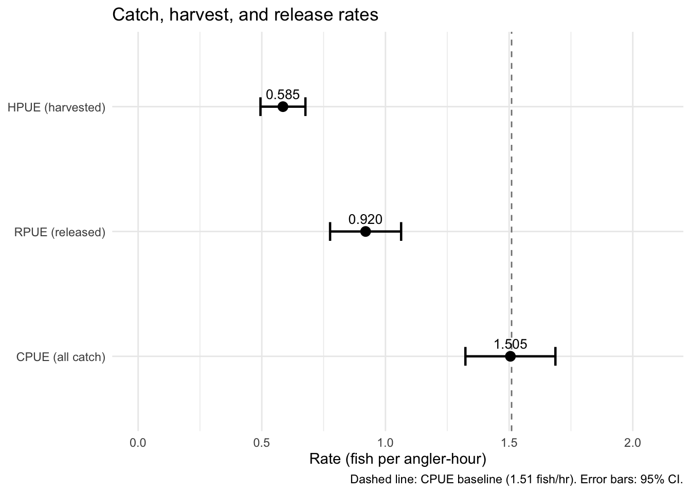
Management decisions often require species-specific catch rates: walleye CPUE is relevant to minimum-size regulations, white bass CPUE to bag limits. estimate_catch_rate(by = species) produces design-based species CPUE with proper stratification weights and confidence intervals:
estimate_catch_rate(harlan_design_ch14, by = species)ℹ Using complete trips for CPUE estimation
(n=390, 65% of 600 interviews) [default]
── Creel Survey Estimates ──────────────────────────────────────────────────────
Method: ratio-of-means-cpue-species
Variance: Taylor linearization
Confidence level: 95%
Grouped by: species
Unit: fish/angler-hour

# A tibble: 11 × 6
   species         estimate      se  ci_lower ci_upper     n
   <chr>              <dbl>   <dbl>     <dbl>    <dbl> <int>
 1 Channel Catfish  0.0393  0.00751  0.0246    0.0541    390
 2 Common Carp      0.00231 0.00187 -0.00136   0.00599   390
 3 Crappie          0       0        0         0         390
 4 Freshwater Drum  0.166   0.0301   0.107     0.225     390
 5 Gizzard Shad     0.00324 0.00229 -0.00124   0.00772   390
 6 Muskellunge      0.00278 0.00156 -0.000288  0.00584   390
 7 Northern Pike    0.00324 0.00130  0.000691  0.00579   390
 8 Walleye          0.389   0.0490   0.292     0.485     390
 9 White Bass       0.828   0.0748   0.681     0.974     390
10 Wiper            0.0148  0.00355  0.00785   0.0218    390
11 Yellow Perch     0.0567  0.0147   0.0279    0.0854    390
White bass and walleye dominate the catch rate, consistent with the Harlan fishery’s reputation as a mixed-species reservoir with high white bass density and a targetable walleye population. Freshwater drum, yellow perch, and channel catfish register lower but meaningful rates. Species with near-zero estimates are rarely targeted and largely absent from completed-trip catch records.
The standard errors reflect the same Taylor linearization variance used for overall CPUE. Confidence intervals for rarer species are wide — for common carp and gizzard shad they span zero — because few completed trips report those species, making the ratio estimator unstable. Species-level CPUE is most reliable when a species appears in at least 15–20% of completed trips.
compare_cpue_estimators() runs all three supported CPUE estimators on the same design object and returns a tidy table, making it straightforward to assess estimator sensitivity:
compare_cpue_estimators(harlan_design_ch14)ℹ Using complete trips for CPUE estimation
(n=390, 65% of 600 interviews)
ℹ Using complete trips for CPUE estimation
(n=390, 65% of 600 interviews)Warning: Non-standard combination: use_trips='complete' with estimator='mor'
ℹ MOR typically used with incomplete trips
ℹ You are using MOR on 390 complete trips - consider `estimator =
'ratio-of-means'` for standard complete trip estimationℹ MOR truncation: 3 trips excluded (< 0.5 hours)
ℹ Using complete trips for CPUE estimation
(n=390, 65% of 600 interviews)# A tibble: 3 × 6
cpue_method estimate se ci_lower ci_upper n
* <chr> <dbl> <dbl> <dbl> <dbl> <int>
1 rom 1.51 0.0928 1.32 1.69 390
2 mor 2.02 0.181 1.67 2.38 387
3 regression 1.31 0.114 1.08 1.53 390At Harlan, ROM returns 1.51 fish/hr, regression returns 1.31 (13% below ROM), and MOR returns 2.02 (34% above ROM). The MOR divergence is expected on an access-point design: MOR weights every completed trip equally regardless of duration, so a few short high-catch trips pull the mean upward. ROM and regression — both duration-weighted — agree within 15% of each other.
Ratio-of-means (ROM, default): divides the total catch across all completed trips by the total effort. A single angler catching twenty fish in two hours contributes 20 fish and 2 hours to the numerator and denominator separately. The estimate is pulled toward trips with long effort because they contribute more hours.
Mean-of-ratios (MOR): computes each completed trip’s catch rate independently and then takes the mean. Every trip gets equal weight regardless of duration. MOR is the natural estimator for roving surveys where mid-trip contacts are observations of instantaneous rate; here it is computed on completed trips for comparison.
Regression CPUE: fits a linear model of catch on effort and reads off the slope as the CPUE estimate. It is less sensitive to the few high-effort, high-catch trips that can inflate ROM.
For the Harlan access-point survey, the ROM estimate is the standard reporting value. The MOR and regression estimates are useful robustness checks. Chapter 17 shows a roving survey where MOR is the primary estimator and ROM is the check.
CPUE is a ratio with a numerator (catch) and a denominator (effort). Both components carry uncertainty, and that uncertainty propagates into the ratio. The standard error produced by estimate_catch_rate() reflects that propagation using Taylor linearization.
Several common misinterpretations deserve explicit attention.
CPUE is not abundance. A CPUE of 1.51 fish per angler-hour does not mean there are 1.51 catchable fish per angler-hour of water. Catchability — the probability that a fish is contacted given it is present — varies with gear type, habitat use, season, and fish behavior. Creel surveys do not estimate catchability; they estimate the rate experienced by anglers. Converting CPUE to abundance requires catchability coefficients that are rarely available.
CPUE comparisons require compatible designs. A weekday CPUE from one year is not directly comparable to a weekend CPUE from another year without accounting for stratum composition.
Higher CPUE does not equal better fishing. Anglers may report high CPUE because they targeted a species with dense schooling behavior, fished during a peak season, or changed their technique.
CPUE from completed trips excludes some anglers systematically. The ROM estimator uses only trips that ended before the survey period closed. Anglers who fished past the survey closing time are excluded.
Reporting CPUE honestly means stating the estimator used, the sample size of completed trips, the survey period and strata included, and a confidence interval. A point estimate alone — “anglers caught 1.5 fish per hour” — strips the precision context that distinguishes a well-supported finding from a noisy snapshot.
CPUE is catch divided by effort, expressed as a ratio with an uncertainty estimate. tidycreel implements two estimators: ratio-of-means for completed trips (default) and mean-of-ratios for incomplete trips (diagnostic or roving designs). At Harlan 2022, the overall completed-trip CPUE is 1.51 fish/hr (95% CI: [1.32, 1.69]). Bank anglers show a higher rate than boat anglers, and the complete vs incomplete diagnostic confirms stationarity.
The most important interpretation rule is also the simplest: report CPUE as a rate observed under a specific design, with its confidence interval, for a specific population of anglers in a specific time window.