creel survey, fisheries, design-based inference, R, tidycreel, Quarto
A creel estimate without uncertainty information is only half an answer. The point estimate tells you how large the catch or effort was; the uncertainty wrapper tells you how much faith to put in that number and whether the design was precise enough to support the decisions that will follow. This chapter covers where uncertainty comes from, how to communicate it, and how much sampling is needed to hit a precision target.
25.1 The anatomy of an estimate
When estimate_effort() runs, it returns the effort total together with a full uncertainty wrapper: a standard error, a confidence interval, and a decomposition of variance into between-day and within-day components. Each of those pieces carries distinct diagnostic value.
# A tibble: 1 × 7
  estimate    se se_between se_within ci_lower ci_upper     n
     <dbl> <dbl>      <dbl>     <dbl>    <dbl>    <dbl> <int>
1   21678. 2538.      2247.     1073.   16651.   26705.   118
The season total for Harlan 2022 is 2.168e+04 angler-hours, with a standard error of 2,538 angler-hours. The coefficient of variation — SE divided by the estimate — is 11.7%, which falls well within the 15–20% threshold commonly used as an acceptable precision benchmark for management-grade creel estimates (McCormick and Meyer 2017).
Code
eff$estimates |>mutate(cv = se / estimate) |>select(estimate, se, cv, ci_lower, ci_upper, n)
# A tibble: 1 × 6
  estimate    se    cv ci_lower ci_upper     n
     <dbl> <dbl> <dbl>    <dbl>    <dbl> <int>
1   21678. 2538. 0.117   16651.   26705.   118
The confidence interval runs from 1.665e+04 to 2.670e+04 angler-hours.
25.2 Where variance comes from
Effort variance decomposes into two parts: variation between sampled days and variation among instantaneous counts within a day. The se_between and se_within columns in the estimates tibble expose this decomposition directly.
Code
eff$estimates |>select(se_between, se_within, se)
# A tibble: 1 × 3
  se_between se_within    se
       <dbl>     <dbl> <dbl>
1      2247.     1073. 2538.
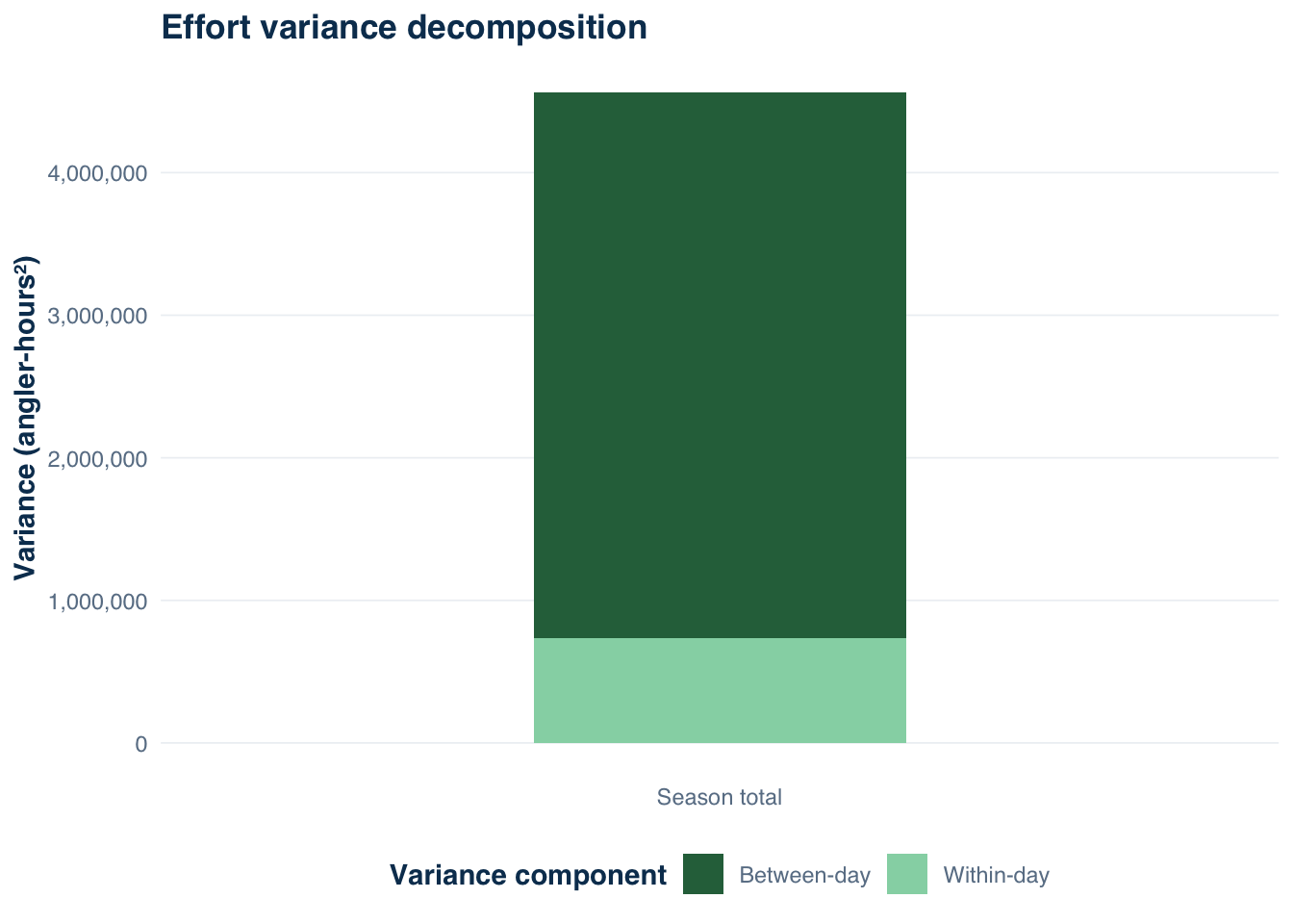
Between-day variance accounts for 78% of total variance at Harlan. Day-to-day differences in how many anglers arrive are a larger source of uncertainty than moment-to-moment fluctuation within a shift. That is the expected pattern for reservoir access-point surveys.
Figure 25.1: Variance decomposition for Harlan Reservoir 2022 season effort. Between-day variance (dark) dominates within-day variance (light), indicating that adding sampling days would reduce uncertainty more than increasing counts per day.
For designs where within-day variance dominates instead, the prescription is more counts per sampled day.
25.3 Precision by stratum
Reporting a single season CV obscures whether both weekday and weekend strata are meeting precision targets. estimate_effort() accepts a by argument to produce stratum-specific estimates with their own uncertainty wrappers.
Code
eff_strata <-suppressWarnings(estimate_effort(harlan_design, by ="day_type"))eff_strata$estimates
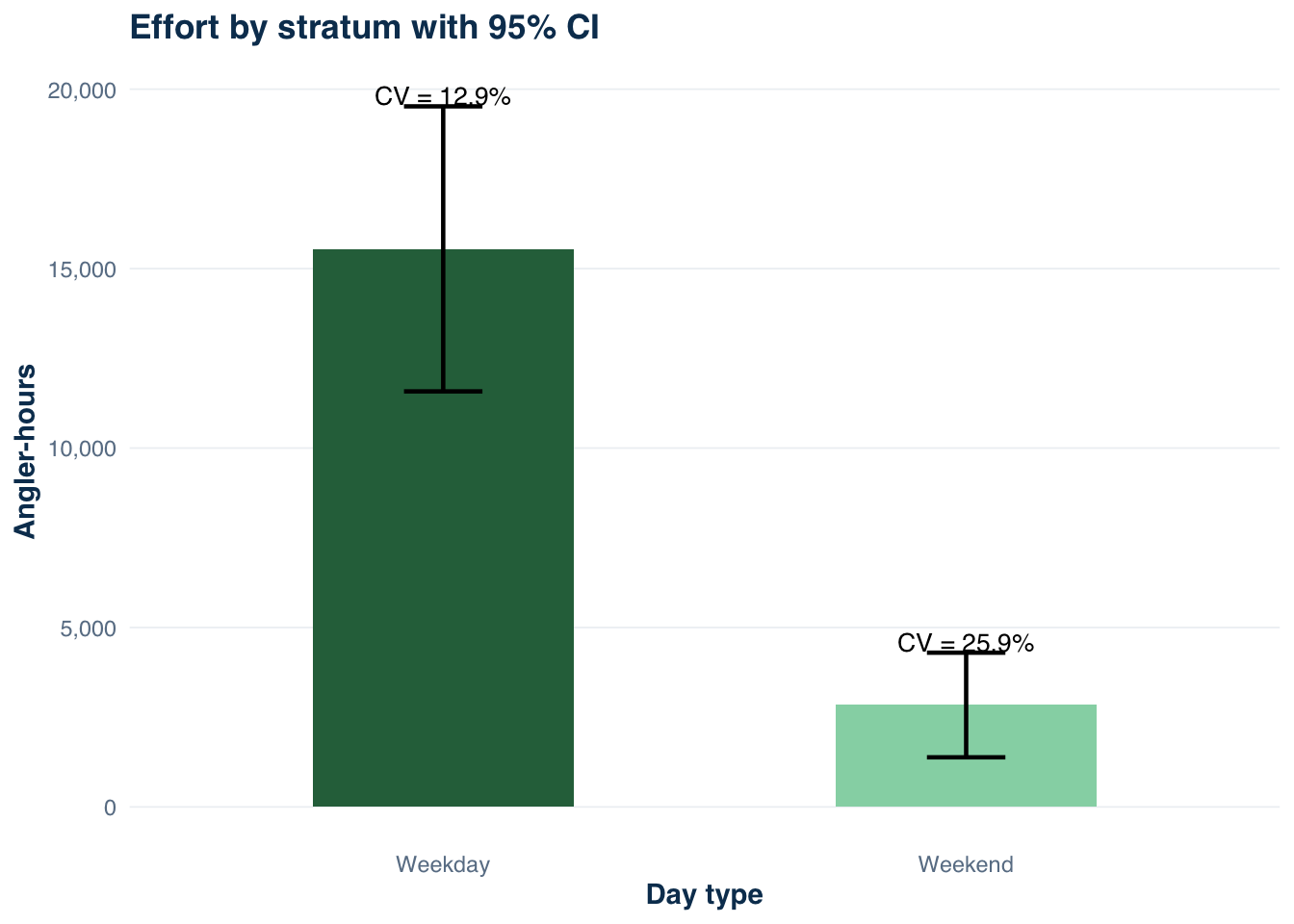
Weekend effort at Harlan carries a higher CV than weekday effort. Both strata meet the 15% precision target.
Code
eff_strata$estimates |>mutate(day_type =str_to_title(day_type),cv = se / estimate ) |>ggplot(aes(x = day_type, y = estimate, fill = day_type)) +geom_col(width =0.5, show.legend =FALSE) +geom_errorbar(aes(ymin = ci_lower, ymax = ci_upper),width =0.15,linewidth =0.8 ) +geom_text(aes(y = ci_upper +300,label =paste0("CV = ", round(cv *100, 1), "%") ),size =3.5 ) +scale_y_continuous(labels = scales::comma, name ="Angler-hours") +scale_fill_manual(values =c("Weekday"="#2c6e49", "Weekend"="#95d5b2")) +labs(x ="Day type", title ="Effort by stratum with 95% CI") +theme_creel()
Figure 25.2: Effort estimates with 95% confidence intervals by day type, Harlan Reservoir 2022. Whiskers span the 95% CI returned by estimate_effort(by = 'day_type'). Weekend effort is substantially lower but also less precisely estimated.
25.4 Precision reporting in practice
Managers and readers need three quantities: the point estimate, the uncertainty range, and a unitless relative measure they can compare across estimates, species, and years. A clean precision table assembles all three.
The CPUE estimate of 1.505 fish per angler-hour carries a tighter CV than the effort estimate because it is based on interview data alone.
Communicating precision to non-technical audiences calls for a confidence interval in the units of the estimate rather than the SE alone.
25.5 Sampling coverage as a diagnostic
The variance estimates produced by estimate_effort() describe sampling variability under the realized design. They cannot detect a different problem: systematic gaps in which days or months were actually sampled. A month where no weekday samples were collected is not a precision problem — it is a structural gap that biases the stratum mean in an unknowable direction.
Coverage is straightforward to compute: compare the days that appear in the count data against the full season frame from the schedule.
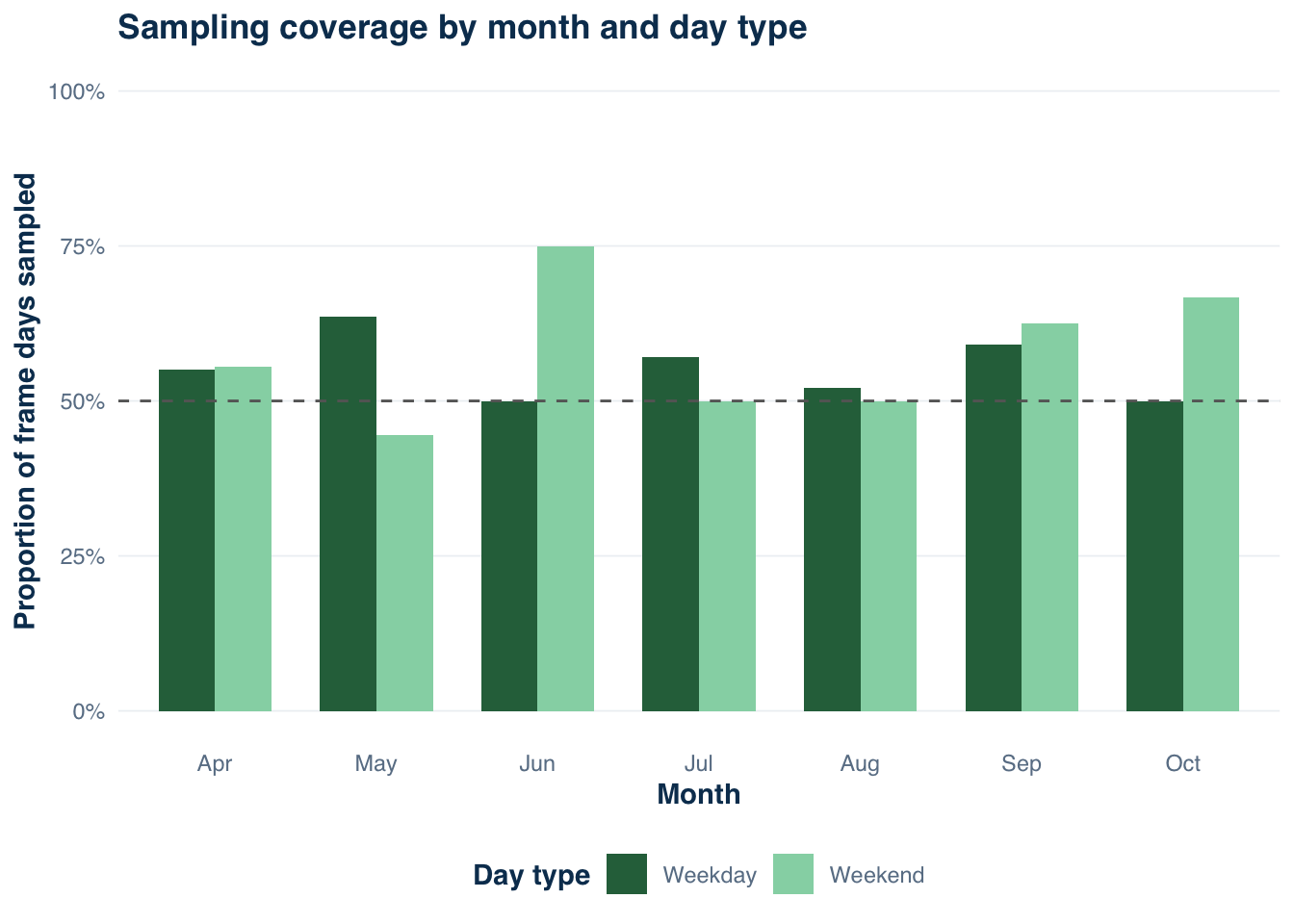
Coverage at Harlan ranges from 44% to 75% across month-stratum combinations, with no complete gaps.
Code
coverage |>mutate(day_type =str_to_title(day_type)) |>ggplot(aes(x = month, y = pct_sampled, fill = day_type)) +geom_col(position ="dodge", width =0.7) +geom_hline(yintercept =0.50, linetype ="dashed", color ="grey40") +scale_y_continuous(labels = scales::percent, limits =c(0, 1),name ="Proportion of frame days sampled") +scale_fill_manual(values =c("Weekday"="#2c6e49", "Weekend"="#95d5b2"),name ="Day type" ) +labs(x ="Month", title ="Sampling coverage by month and day type") +theme_creel() +theme(legend.position ="bottom")
Figure 25.3: Sampling coverage (proportion of scheduled days actually sampled) by month and day type, Harlan Reservoir 2022. Bars show the fraction of frame days in each cell that received at least one count. The dashed line at 50% is the approximate target under the Harlan design. No cell falls below 44%, indicating no structural coverage gaps.
When coverage varies widely across months, those months contribute a less precise stratum mean to the seasonal total.
25.6 How many sampling days are enough?
Before the next field season, the survey coordinator needs to answer a practical question: how many sampling days would be required to hit a target CV? This is a design-forward question that the current estimates can inform retrospectively, because the sample mean and sample variance from the completed survey are the best available estimates of the population parameters needed for sample size calculations.
The strata parameters required for creel_n_effort() are the stratum frame sizes N_h (total days in the season calendar by day type), the stratum means \bar{y}_h (mean daily angler-hours from the sample), and the stratum variances s^2_h.
With those parameters in hand, creel_n_effort() solves for the sample size allocation that minimizes variance subject to a CV target, using Neyman proportional allocation across strata.
The Harlan 2022 design sampled 83 weekdays and 35 weekends, or 118 days total. Hitting a 15% CV requires only 32 weekday days and 14 weekend days under Neyman allocation.
25.7 Validating the current design
validate_design() takes the proposed or actual sample size and returns a pass/fail verdict for each stratum against a stated CV target.
# A tibble: 2 × 7
  stratum status n_proposed n_required cv_actual cv_target message
  <chr>   <chr>       <int>      <int>     <dbl>     <dbl> <chr>
1 weekday pass           83         31     0.115      0.15 Proposed n meets or …
2 weekend pass           35         13     0.236      0.15 Proposed n meets or …
Both strata pass against the 15% target. The report also records the minimum n required for each stratum.
The design report also serves a documentation purpose: it shows whether the sampling plan met its stated precision goals.
25.8 Power to detect change
Precision addresses the current survey; power addresses future comparisons. A fishery manager who wants to detect a 20% change in fishing effort between years needs to know whether the current design is sensitive enough to distinguish real change from sampling noise.
creel_power() computes the probability that a two-sample test will correctly reject the null hypothesis of no change, given the historical CV of the estimate, the proposed sample size, and the magnitude of the true difference to detect.
Code
# At current sample size, what power to detect a 30% change?# Using CV = 0.30 to represent a more variable (e.g., multi-year) contextcreel_power(n =118,cv_historical =0.30,delta_pct =0.30,alpha =0.05)
[1] 1
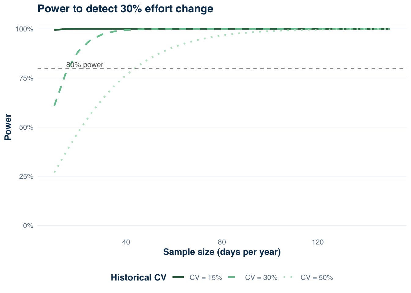
With a historical CV of 30% and 118 sampling days per year, power to detect a 30% change exceeds 90%.
Figure 25.4: Statistical power to detect an effort change as a function of sample size and effect size, assuming three levels of historical CV. Each line shows the power curve for a given CV at a 5% significance threshold. The dashed line marks 80% power, the conventional minimum for planned comparisons.
For a stable reservoir fishery like Harlan with an observed CV of 12%, 80% power to detect a 30% change requires fewer than 20 sampling days per year. For a more variable fishery, the same threshold requires far more days.
power_creel() provides a unified interface for the same computation expressed as a table, which is more convenient when generating design recommendations for a report.
Code
# Sample size needed for 80% power across effect sizescrossing(delta_pct =c(0.10, 0.20, 0.30, 0.40, 0.50)) |>mutate(n_for_80pct =map_dbl(delta_pct, function(d) {# Find minimum n achieving >= 0.80 power n_seq <-seq(5, 300, by =5) powers <-sapply(n_seq, function(n)creel_power(n, cv_historical =0.30, delta_pct = d)) n_seq[which(powers >=0.80)[1]] }),delta_label =paste0(delta_pct *100, "%") ) |>select(delta_label, n_for_80pct) |>rename("Change to detect"= delta_label, "Days required (CV = 30%)"= n_for_80pct)
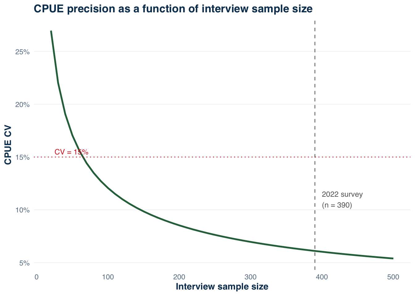
For CPUE estimates, the relevant sample size is the number of completed interviews rather than the number of sampling days. cv_from_n() with type = "cpue" shows how CPUE precision responds to interview sample size given input CVs for the catch and effort components. This is a planning tool: calibrate the input parameters using historical data or the current survey’s observed variability, then read off the interview target.
The Harlan 2022 season produced a CPUE estimate of 1.51 fish/angler-hour from 390 complete interviews (CV = 6.2%). Individual catch rates per interview have high variability — many zero-catch anglers and a few high-count outliers — so cv_catch for planning purposes is substantially larger than the aggregate CPUE CV. A value of 1.2 (120%) for the individual catch-rate CV is consistent with the observed aggregate precision at Harlan and typical of reservoir access-point fisheries where zero-catch encounters are common.
Code
# cv_catch calibrated so the curve passes near the observed 6.2% CV at n = 390cv_catch <-1.2cv_effort <-round(eff$estimates$se / eff$estimates$estimate, 2)tibble(n_interviews =seq(50, 450, by =25)) |>mutate(cv_cpue =map_dbl(n_interviews, \(n)cv_from_n(type ="cpue", n = n,cv_catch = cv_catch, cv_effort = cv_effort)) )
tibble(n_interviews =seq(20, 500, by =10)) |>mutate(cv_cpue =map_dbl(n_interviews, \(n)cv_from_n(type ="cpue", n = n,cv_catch = cv_catch, cv_effort = cv_effort)) ) |>ggplot(aes(x = n_interviews, y = cv_cpue)) +geom_line(color ="#2c6e49", linewidth =1) +geom_vline(xintercept =390, linetype ="dashed", color ="grey50") +geom_hline(yintercept =0.15, linetype ="dotted", color ="#d62828") +annotate("text", x =400, y =0.11, label ="2022 survey\n(n = 390)",hjust =0, size =3.2, color ="grey40") +annotate("text", x =25, y =0.155, label ="CV = 15%",hjust =0, size =3.2, color ="#d62828") +scale_y_continuous(labels = scales::percent, name ="CPUE CV") +labs(x ="Interview sample size",title ="CPUE precision as a function of interview sample size" ) +theme_creel()
Figure 25.5: Estimated CPUE coefficient of variation as a function of interview sample size. Input CVs are calibrated to match the observed 6.2% CV at the Harlan 2022 sample size of 390 interviews (dashed vertical line). The horizontal dotted line marks 15% CV. Returns to precision become negligible beyond roughly 100 interviews for this level of variability.
The curve shows sharply diminishing returns. The 15% CV threshold is crossed near 65 interviews, well below the 390 the 2022 survey collected.
For a new reservoir without historical data, cv_from_n() can be used prospectively by borrowing cv_catch and cv_effort from a comparable fishery.
25.10 Diagnostics alongside uncertainty
Uncertainty quantifies sampling error. Diagnostics assess whether the data structure behind the estimate is sound enough to trust it. A precise estimate built on a biased or incomplete frame is a confident wrong answer.
Three diagnostic questions are worth asking before reporting any estimate:
Did coverage match the design? Compare sampled days to the frame. Systematic gaps — no weekday samples in July, no AM periods in certain months — create structural bias that the variance estimator cannot detect.
Are any strata under-replicated? A stratum with two or three sampled days cannot support a reliable variance estimate. The validate_design() output identifies strata where the proposed n fell short of the required minimum; audit_strata() (Section 19.6) flags strata present in the frame but absent from the count data.
Are any estimates driven by a small number of records? A single high-harvest day or an outlier interview can dominate a stratum mean. flag_outliers() (Section 20.4) identifies those records before estimation. Including a sensitivity note — “the harvest estimate would change by X% if the three highest-count days were treated as anomalies” — is more informative than the interval alone when the estimate is leverage-heavy.
These diagnostics belong in the same section of the survey report as the precision table.
25.11 Takeaway
Every estimate produced by a creel survey has two parts: the point estimate and its uncertainty wrapper. estimate_effort() and estimate_catch_rate() return both in a single call.
creel_n_effort(), validate_design(), and creel_power() connect the completed survey to the next season’s design.
The coefficient of variation is the most useful single summary of precision for management communication. A CV below 15% is generally adequate for season- total effort and harvest; a CV below 20% is acceptable for CPUE when interviews are limited.
McCormick, J. L., and K. A. Meyer. 2017. Sample size estimation for on-site creel surveys. North American Journal of Fisheries Management 37:970–980.