25  Reporting and Interpretation

Keywords

creel survey, fisheries, design-based inference, R, tidycreel, Quarto

25.1 Reporting as the final mile

A creel survey produces estimates with standard errors and confidence intervals. Whether those numbers serve their purpose depends entirely on how they are communicated. A well-executed survey can mislead if the report fails to state what domain was sampled, how the estimate was constructed, or what uncertainty attaches to the result. A less precise survey can still support a sound management decision if the report is honest about its limitations and what the numbers cannot answer.

Reporting is not cleanup that happens after analysis — it is the last step of analysis. The decisions made during survey design (which strata to sample, which estimator to apply, which interviews to include) determine what the final number actually measures. The report is where those decisions become visible to people who did not make them. A number without a domain statement is not an estimate; it is a quantity of unknown scope.

This chapter shows how to assemble all Harlan Reservoir 2022 estimates into a single report-ready structure, write defensible narrative sentences with inline R so the prose stays synchronized with the analysis, present tables and figures appropriate for different management audiences, and state caveats that protect readers from overgeneralizing results to domains the survey did not cover.

25.2 The reporting contract

Every creel report makes an implicit claim about what the numbers mean. Making that claim explicit requires six elements, stated in some form before any estimates appear.

1. The question. What biological or management quantity was the primary target? Effort, total harvest, catch rate, or all three? Specifying the question first tells the reader what to look for and what to skip. A report whose stated question is “what was the total harvest of game fish at Harlan Reservoir in 2022?” has a different burden of evidence than one asking “how did effort vary by day type?”

2. The domain. Which part of the fishery do the estimates cover? The Harlan 2022 survey sampled public-access areas using an access-point design during standard operating hours from April through October. Estimates therefore apply to that spatiotemporal domain — not to private shorelines, not to pre-spawn April activity occurring before sampling began, not to effort on days when no crew was deployed.

The most common reporting failure is leaving the domain unstated (Pollock et al. 1994). Without it, an estimate of 19,000 fish harvested reads as though it applies to the entire reservoir and the entire calendar year. It does not. The domain is not a caveat to be buried at the end — it belongs in the same sentence as the number.

3. The design and unit of analysis. Stratified access-point creel survey; day-type strata (weekday and weekend); angler-hours as the effort unit; party-based interviews; 600 total interviews across the season. A reader who understands the design can evaluate whether the estimators are appropriate and whether the same design could be applied to their own system.

4. The key estimates. Point estimates for each quantity, with labels that include units. “Effort” is ambiguous; “33,000 angler-hours” is not.

5. Uncertainty. Standard errors and 95% confidence intervals for every estimate in the report. A point estimate without uncertainty is not an estimate — it is a guess with no information about how seriously to take it. Presenting only the point estimate implicitly claims perfect precision, which no creel survey achieves.

6. Interpretation. A brief statement of what the estimate implies for management, constrained to what the data can support. The interpretation should not be wider than the domain. If the survey covered public-access areas only, the interpretation should not conclude that the total fishery is under pressure — it should conclude that the sampled portion shows evidence of pressure.

These six elements protect both the reader and the analyst. Readers get the information they need to evaluate how much weight to put on the numbers. Analysts get a record of what the survey was designed to measure and a defense against future questions about what was or was not estimated.

25.3 Assembling the Harlan estimates

Chapters 12 through 15 demonstrated each estimator separately. A report needs all of them together, in one structure, so that the full picture of the fishery is visible at once. The starting point is the same design object built throughout Part IV — here reconstructed from the raw Harlan data in a hidden setup chunk using the same pipeline from those earlier chapters.

Running all estimates in sequence and extracting the $estimates slot from each produces a set of tibbles with a consistent column structure: estimate, se, ci_lower, ci_upper. That structural consistency is what makes assembly straightforward.

eff_ch16     <- estimate_effort(harlan_design_ch16,         target = "stratum_total")

Warning: Count variable angler_hours contains 18 zero values.
ℹ Zero values may indicate days with no fishing activity or data collection
  issues.
ℹ Consider whether zeros are true zeros or missing data.

harvest_ch16 <- estimate_total_harvest(harlan_design_ch16,  target = "stratum_total")
catch_ch16   <- estimate_total_catch(harlan_design_ch16,    target = "stratum_total")
release_ch16 <- estimate_total_release(harlan_design_ch16,  target = "stratum_total")
cpue_ch16    <- estimate_catch_rate(harlan_design_ch16)

ℹ Using complete trips for CPUE estimation
  (n=390, 65% of 600 interviews) [default]

hpue_ch16    <- estimate_harvest_rate(harlan_design_ch16)

ℹ Filtering to complete trips for HPUE estimation
  (n=390, 65% of 600 interviews) [default]

rpue_ch16    <- estimate_release_rate(harlan_design_ch16)

ℹ Filtering to complete trips for RPUE estimation
  (n=390, 65% of 600 interviews) [default]

The target = "stratum_total" argument expands sampled-day estimates to the full stratum — the appropriate choice when reporting a season total rather than a summary of surveyed days only. The rate estimators (estimate_catch_rate, estimate_harvest_rate, estimate_release_rate) do not take a target argument because they are ratios, not totals; they are already expressed per unit effort and scale-free with respect to sampling intensity.

With all seven objects in hand, bind_rows() collects them into a single reporting table. A select() call standardizes the column set across estimators that return slightly different output structures (effort returns se_between and se_within; other estimators return only se).

report_summary <- bind_rows(
  eff_ch16$estimates |>
    select(estimate, se, ci_lower, ci_upper) |>
    mutate(quantity = "Effort",         unit = "angler-hours"),
  harvest_ch16$estimates |>
    select(estimate, se, ci_lower, ci_upper) |>
    mutate(quantity = "Total harvest",  unit = "fish"),
  catch_ch16$estimates |>
    select(estimate, se, ci_lower, ci_upper) |>
    mutate(quantity = "Total catch",    unit = "fish"),
  release_ch16$estimates |>
    select(estimate, se, ci_lower, ci_upper) |>
    mutate(quantity = "Total release",  unit = "fish"),
  cpue_ch16$estimates |>
    select(estimate, se, ci_lower, ci_upper) |>
    mutate(quantity = "CPUE",           unit = "fish / hr"),
  hpue_ch16$estimates |>
    select(estimate, se, ci_lower, ci_upper) |>
    mutate(quantity = "HPUE",           unit = "fish / hr"),
  rpue_ch16$estimates |>
    select(estimate, se, ci_lower, ci_upper) |>
    mutate(quantity = "RPUE",           unit = "fish / hr")
) |>
  select(quantity, unit, estimate, se, ci_lower, ci_upper)

report_summary

# A tibble: 7 × 6
  quantity      unit          estimate        se  ci_lower  ci_upper
  <chr>         <chr>            <dbl>     <dbl>     <dbl>     <dbl>
1 Effort        angler-hours 33052.    3704.     25716.    40388.   
2 Total harvest fish         19825.    2635.     14649.    25000.   
3 Total catch   fish         49756.    6349.     37272.    62239.   
4 Total release fish         30310.    4129.     22201.    38419.   
5 CPUE          fish / hr        1.51     0.0928     1.32      1.69 
6 HPUE          fish / hr        0.585    0.0464     0.495     0.676
7 RPUE          fish / hr        0.920    0.0733     0.776     1.06 

The seven-row tibble is the raw material for every derived output in this chapter — narrative sentences, formatted tables, and all three figures. All downstream objects read from report_summary or from the individual estimate objects, so any change to the estimation pipeline propagates automatically.

The estimates confirm the values established in earlier chapters: 33,052 angler-hours of effort, 19,825 fish harvested, 49,756 fish caught in total, and a catch rate of 1.51 fish per angler-hour. The harvest CI spans from 14,649 to 25,000 fish — a range of 10,350 fish from lower to upper bound. Reporting only the point estimate would conceal that entire span.

25.4 Narrative reporting with inline R

A table of estimates is not a report. It is the evidence a report draws on. The report also needs to tell the reader what the estimates mean, in plain language, with the numbers embedded directly in the prose so that a reader who never reaches the table still encounters the key result.

Quarto supports inline R expressions using backtick notation: any expression inside `r ` is evaluated at render time and its result is inserted into the surrounding prose. This mechanism ensures that the narrative cannot drift from the analysis. If the data or design changes, re-rendering the document updates every inline number automatically. There is no manual transcription step where errors can enter.

fmt_comma <- function(x) formatC(round(x), format = "f", digits = 0, big.mark = ",")
fmt_rate  <- function(x) sprintf("%.2f", x)
fmt_pct   <- function(x) sprintf("%.1f%%", x)

These helpers, defined once in the setup chunk, cover the three formats that creel reports need most often. fmt_comma() rounds to the nearest integer and adds thousand-separator commas — appropriate for totals where sub-unit precision is spurious. fmt_rate() uses two decimal places — appropriate for CPUE and HPUE where differences at the second decimal place can signal meaningful change across years. fmt_pct() formats coefficients of variation as percentages for precision tables.

The sentence pattern that works for creel estimates has three parts: what was estimated, how large the estimate is, and how uncertain it is. Domain belongs in the first part. The three examples below show correctly structured report sentences for effort, harvest, and catch rate.

NoteReport sentence: effort

Anglers expended an estimated 33,052 angler-hours at Harlan Reservoir during the 2022 open season (95% CI: 25,716–40,388 angler-hours).

NoteReport sentence: harvest

Total harvest in public-access areas was estimated at 19,825 fish (SE = 2,635, 95% CI: 14,649–25,000 fish).

NoteReport sentence: catch rate

The overall catch rate was 1.51 fish per angler-hour (SE = 0.09, 95% CI: 1.32–1.69 fish / hr), based on 390 completed party interviews.

Each sentence includes the domain, the unit, and the uncertainty.

Choosing precision is also a reporting decision. Rounding to the nearest hundred or even the nearest thousand is defensible for a management report.

harvest_est <- harvest_ch16$estimates$estimate

cat(sprintf(
  "Raw point estimate:       %s fish\n
Rounded to nearest 100:   %s fish\n
Rounded to nearest 1,000: %s fish\n",
  fmt_comma(harvest_est),
  fmt_comma(round(harvest_est, -2)),
  fmt_comma(round(harvest_est, -3))
))

Raw point estimate:       19,825 fish

Rounded to nearest 100:   19,800 fish

Rounded to nearest 1,000: 20,000 fish

For most management contexts, rounding to the nearest hundred preserves the meaningful information while avoiding spurious precision. The exact rounding choice should be stated in the report — “estimates are rounded to the nearest 100 fish” — so readers understand that the reported figure is not exact.

25.5 The summary table

A formatted summary table presents all estimates simultaneously with consistent rounding and visible uncertainty. The goal is a table that a fisheries manager can hand to a supervisor or include in an annual report without additional editing.

report_table <- report_summary |>
  mutate(
    Estimate = case_when(
      unit %in% c("angler-hours", "fish") ~ fmt_comma(estimate),
      TRUE                                 ~ fmt_rate(estimate)
    ),
    SE = case_when(
      unit %in% c("angler-hours", "fish") ~ fmt_comma(se),
      TRUE                                 ~ fmt_rate(se)
    ),
    `95% CI` = paste0(
      case_when(
        unit %in% c("angler-hours", "fish") ~ fmt_comma(ci_lower),
        TRUE                                 ~ fmt_rate(ci_lower)
      ),
      "–",
      case_when(
        unit %in% c("angler-hours", "fish") ~ fmt_comma(ci_upper),
        TRUE                                 ~ fmt_rate(ci_upper)
      )
    ),
    CV = fmt_pct(se / estimate * 100)
  ) |>
  select(
    Quantity = quantity,
    Unit     = unit,
    Estimate,
    SE,
    `95% CI`,
    CV
  )

report_table

# A tibble: 7 × 6
  Quantity      Unit         Estimate SE    `95% CI`      CV   
  <chr>         <chr>        <chr>    <chr> <chr>         <chr>
1 Effort        angler-hours 33,052   3,704 25,716–40,388 11.2%
2 Total harvest fish         19,825   2,635 14,649–25,000 13.3%
3 Total catch   fish         49,756   6,349 37,272–62,239 12.8%
4 Total release fish         30,310   4,129 22,201–38,419 13.6%
5 CPUE          fish / hr    1.51     0.09  1.32–1.69     6.2% 
6 HPUE          fish / hr    0.59     0.05  0.49–0.68     7.9% 
7 RPUE          fish / hr    0.92     0.07  0.78–1.06     8.0% 

The CV column — coefficient of variation, expressed as SE / estimate × 100 — gives readers a scale-free precision indicator. A CV below 20% is commonly cited as management-grade precision for recreational fisheries surveys (Pollock et al. 1994).

The table should appear in any report with a caption that states the domain.

25.6 Summary figure: totals

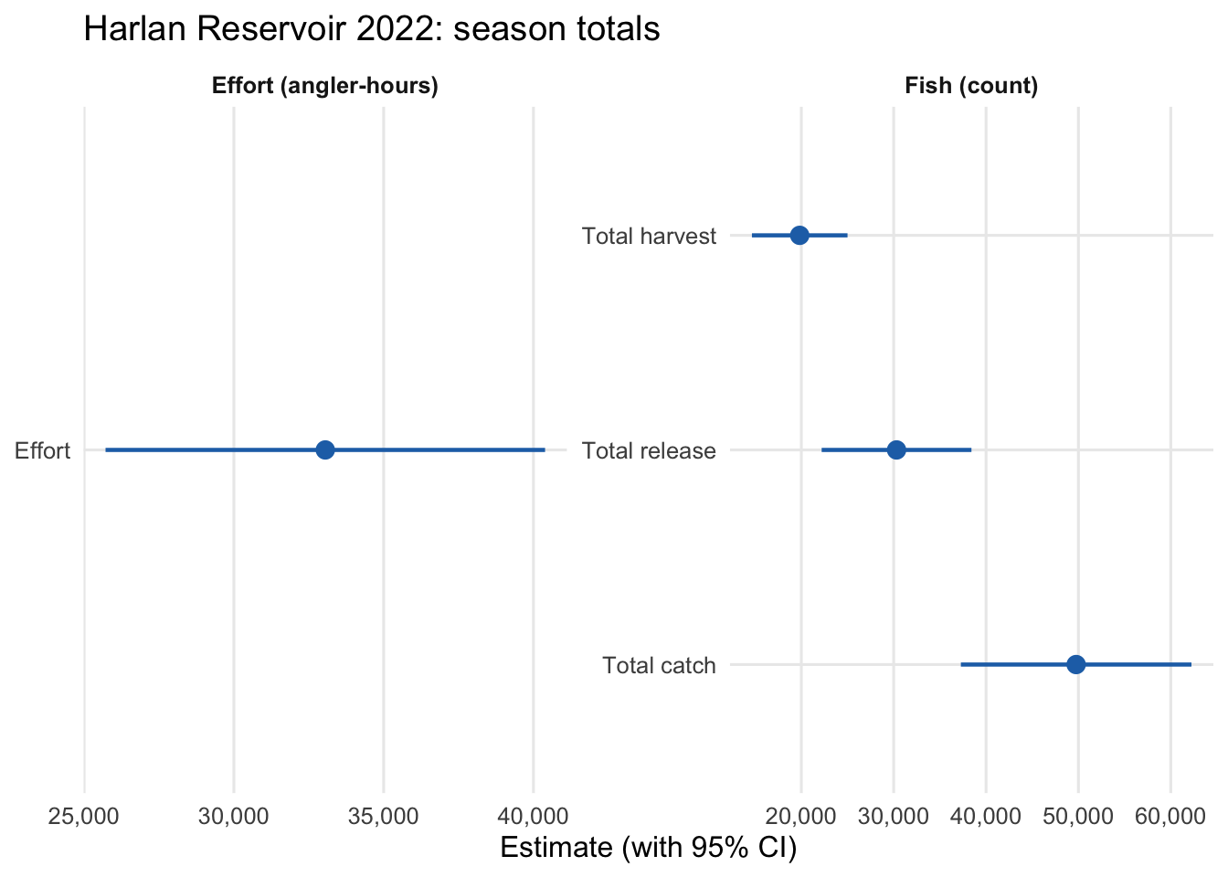
For audiences who read figures before tables, a summary plot that shows all totals with confidence intervals communicates scale and uncertainty more efficiently than a table. Because effort (angler-hours) and the fish counts (harvest, catch, release) have different units and very different magnitudes, they require separate panels with free scales.

totals_effort <- report_summary |>
  filter(quantity == "Effort") |>
  mutate(panel = "Effort (angler-hours)")

totals_fish <- report_summary |>
  filter(quantity %in% c("Total catch", "Total harvest", "Total release")) |>
  mutate(panel = "Fish (count)")

totals_plot <- bind_rows(totals_effort, totals_fish) |>
  mutate(
    quantity = fct_relevel(quantity, "Total catch", "Total release", "Total harvest"),
    panel    = fct_relevel(panel, "Effort (angler-hours)", "Fish (count)")
  )

ggplot(totals_plot, aes(x = estimate, y = quantity)) +
  geom_linerange(
    aes(xmin = ci_lower, xmax = ci_upper),
    linewidth = 0.8,
    color     = "#2171b5"
  ) +
  geom_point(
    size  = 3,
    color = "#2171b5"
  ) +
  scale_x_continuous(labels = scales::comma) +
  facet_wrap(~panel, scales = "free", ncol = 2) +
  labs(
    x     = "Estimate (with 95% CI)",
    y     = NULL,
    title = "Harlan Reservoir 2022: season totals"
  ) +
  theme_minimal(base_size = 12) +
  theme(
    strip.text       = element_text(face = "bold"),
    panel.grid.minor = element_blank()
  )

Figure 25.1: Season totals for Harlan Reservoir 2022. Left panel: total angling effort in angler-hours. Right panel: estimated total catch, harvest, and release in number of fish. Points are ratio-of-means estimates; horizontal bars show 95% confidence intervals. Catch exceeds harvest because the majority of fish were released; the CI on each total reflects combined uncertainty from effort estimation and rate estimation.

The width of the confidence intervals in both panels conveys that the estimates carry meaningful uncertainty.

25.7 Precision profile

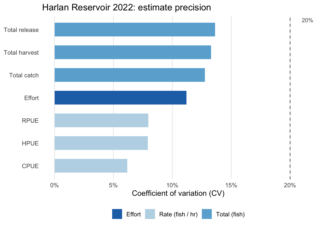
Not all estimates from the same survey are equally reliable. A precision profile makes those differences visible.

cv_tbl <- report_summary |>
  mutate(cv = se / estimate * 100) |>
  mutate(
    quantity = fct_reorder(quantity, cv),
    category = case_when(
      quantity == "Effort"                              ~ "Effort",
      as.character(quantity) %in% c("Total harvest",
                                    "Total catch",
                                    "Total release")   ~ "Total (fish)",
      TRUE                                              ~ "Rate (fish / hr)"
    )
  )

ggplot(cv_tbl, aes(x = cv, y = quantity, fill = category)) +
  geom_col(width = 0.6) +
  geom_vline(xintercept = 20, linetype = "dashed", color = "gray40") +
  annotate(
    "text",
    x = 21, y = Inf,
    label    = "20% target",
    hjust    = 0,
    vjust    = 1.5,
    size     = 3.2,
    color    = "gray30"
  ) +
  scale_fill_manual(
    values = c(
      "Effort"           = "#2171b5",
      "Total (fish)"     = "#6baed6",
      "Rate (fish / hr)" = "#bdd7e7"
    )
  ) +
  scale_x_continuous(labels = function(x) paste0(x, "%")) +
  labs(
    x    = "Coefficient of variation (CV)",
    y    = NULL,
    fill = NULL,
    title = "Harlan Reservoir 2022: estimate precision"
  ) +
  theme_minimal(base_size = 12) +
  theme(
    legend.position    = "bottom",
    panel.grid.minor   = element_blank(),
    panel.grid.major.y = element_blank()
  )

Figure 25.2: Coefficient of variation (CV) for each Harlan Reservoir 2022 estimate. Bars show SE / estimate × 100. The dashed vertical line at 20% marks a commonly cited threshold for management-grade precision in recreational fishery surveys. Estimates with CVs above 20% should be interpreted cautiously and may justify increased sampling effort in future seasons.

For the Harlan 2022 survey, effort precision (CV = 11.2%) falls within the range expected for a stratified access-point survey with adequate sampling of both day types. Harvest carries a substantially higher CV (CV = 13.3%) because it inherits uncertainty from both the effort expansion and the harvest rate estimation; each source of uncertainty combines multiplicatively in the total. The catch rate, derived only from completed trip interviews, has a CV of 6.2% — moderate precision that reflects the number of completed interviews relative to the variability in individual catch outcomes.

Estimates that exceed the 20% CV threshold are not wrong — they are imprecise. An imprecise estimate is still useful if the management question is whether a quantity is large or small, not whether it equals a specific value. An estimated harvest with a high CV still rules out both very low and very high harvests; it just cannot distinguish between values that differ by less than about one standard error on either side of the point estimate.

If specific estimates consistently fall above the CV threshold across years, the appropriate response is to revisit the sampling design rather than to report the numbers without comment. Section 24.6 and Section 24.8 showed how creel_power() and cv_from_n() can guide sample size decisions toward a precision target. The precision profile here identifies which quantities need that investment.

25.8 Stratified reporting

The season totals are the headline, but stratified estimates often contain the management-relevant signal. A regulation that differentially affects weekday or weekend fishing — a bag limit change, a closure, a catch-and-release requirement — should be evaluated against stratified estimates, not the pooled season total.

The same estimate_total_harvest() call with a by argument produces stratum-level estimates. These share the design structure from the overall call, so the stratified and unstratified results are methodologically consistent.

harvest_by_dt <- estimate_total_harvest(
  harlan_design_ch16,
  by     = day_type,
  target = "stratum_total"
)

harvest_by_dt$estimates

# A tibble: 2 × 6
  day_type estimate    se ci_lower ci_upper     n
  <chr>       <dbl> <dbl>    <dbl>    <dbl> <int>
1 weekday    15793. 2346.   11186.   20400.   489
2 weekend     4032. 1200.    1675.    6389.   111

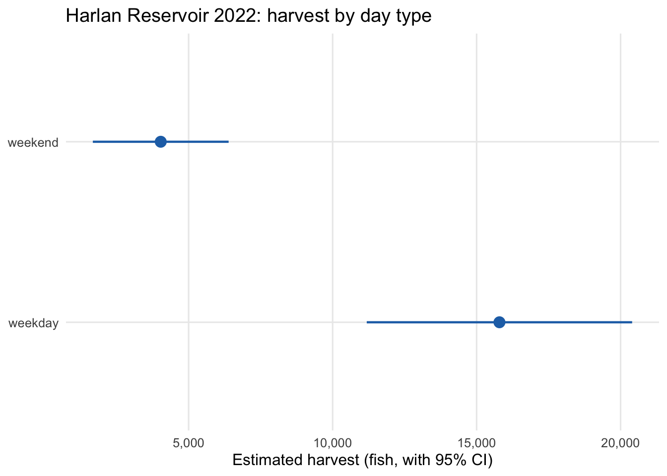
The stratified harvest figures answer a question the season total cannot: where does the removal occur? A figure makes the comparison immediate.

ggplot(harvest_by_dt$estimates, aes(x = estimate, y = day_type)) +
  geom_linerange(
    aes(xmin = ci_lower, xmax = ci_upper),
    linewidth = 0.8,
    color     = "#2171b5"
  ) +
  geom_point(size = 3.5, color = "#2171b5") +
  scale_x_continuous(labels = scales::comma) +
  labs(
    x     = "Estimated harvest (fish, with 95% CI)",
    y     = NULL,
    title = "Harlan Reservoir 2022: harvest by day type"
  ) +
  theme_minimal(base_size = 12) +
  theme(panel.grid.minor = element_blank())

Figure 25.3: Estimated total harvest by day type at Harlan Reservoir, 2022. Points show stratum-total estimates; bars show 95% confidence intervals. Weekday harvest substantially exceeds weekend harvest in absolute terms because the weekday stratum contains more days and accumulated more angler-hours over the season.

strat_table <- harvest_by_dt$estimates |>
  mutate(
    `Day type` = day_type,
    Harvest    = fmt_comma(estimate),
    SE         = fmt_comma(se),
    `95% CI`   = paste0(fmt_comma(ci_lower), "–", fmt_comma(ci_upper)),
    CV         = fmt_pct(se / estimate * 100)
  ) |>
  select(`Day type`, Harvest, SE, `95% CI`, CV)

strat_table

# A tibble: 2 × 5
  `Day type` Harvest SE    `95% CI`      CV   
  <chr>      <chr>   <chr> <chr>         <chr>
1 weekday    15,793  2,346 11,186–20,400 14.9%
2 weekend    4,032   1,200 1,675–6,389   29.8%

The stratified harvest table answers a different question than the season total: not how many fish were harvested overall, but whether harvest is concentrated in weekday or weekend fishing. That distinction matters when a regulation change would close or restrict one day type, because the season-total reduction is not proportional to harvest per day — it depends on how many days of each type occur and how much harvest each carries.

Interpreting stratified estimates correctly requires stating the stratum definition in the table caption. “Weekday” in the Harlan survey means any Monday through Friday that fell within the sampling frame; “weekend” means Saturday and Sunday. A regulation effective only on Saturdays would affect a subset of the “weekend” stratum, and the stratum estimate would overstate the impact unless further post-stratified.

25.9 Domain and scope

Every estimate has a scope boundary. The boundary is not a limitation to apologize for — it is a property of the design that tells readers where the estimate applies. Stating it clearly prevents two common errors: applying the estimate to a domain it cannot cover, and assuming the estimate is invalid because it does not cover everything.

For the Harlan 2022 survey, the scope boundaries are:

Temporal scope. Sampling ran from April through October during standard crew operating hours. Effort and harvest on days outside the sampling frame, during pre-dawn and late-evening hours, and on crew non-deployment days are not in the estimate. Winter fishing is excluded entirely.

Spatial scope. The access-point design covers public-access areas where departing anglers can be intercepted. Private shorelines, mid-lake boats not associated with a sampled access point, and tributaries outside the main reservoir are not represented.

Species scope. Catch and harvest rates are available for species recorded in the catch table. Rare species may be under-sampled — a catch record requires that at least one party in the interview sample encountered that species. Total harvest by species inherits both effort uncertainty and the sampling uncertainty from the catch table.

Design scope. The access-point method samples anglers as they depart. It is not designed to capture effort by anglers who never return to a sampled access point (e.g., anglers who enter by canoe and exit via a private road). The fraction of effort in those groups is unknown; if it is large, the effort estimate is biased downward.

Stating these boundaries in the report is the information a reader needs to decide whether the estimate answers their question.

25.10 Writing for different audiences

A creel report often serves audiences with different needs and different tolerances for statistical language. Field staff need operational feedback. Managers need a decision summary. Researchers need methodological detail. Stakeholders need a plain-language explanation of what the survey found.

The same estimates can support all four audiences without changing the claim.

Manager summary (2–3 sentences). Lead with the most policy-relevant quantity. State the estimate, the CI, and one interpretive sentence.

NoteManager version

The 2022 Harlan Reservoir creel survey estimated 19,825 fish harvested (95% CI: 14,649–25,000) from public-access areas during the April–October season. The catch rate of 1.51 fish per angler-hour was within the range observed in recent years. Total effort was approximately 33,052 angler-hours.

Researcher disclosure. Provide the estimator name, the variance formula, the software pipeline, and any assumptions that were checked or violated. State CV for each quantity and note any diagnostic findings (incomplete-trip sensitivity, variance decomposition, coverage diagnostics). The report_table from Section 25.5, with its CV column, is the core of a researcher-facing results section.

Stakeholder language. Avoid jargon, define every number in plain terms before stating it, and lead with what the fishery looked like rather than what the survey was designed to do.

NoteStakeholder version

About 19,825 fish were kept by anglers fishing Harlan Reservoir in 2022. That number could be anywhere from 14,649 to 25,000 fish, depending on how representative the surveyed days were of the full season. Of all fish caught, roughly 60.2% were released.

The estimate does not change between these versions. What changes is which information gets foregrounded and what vocabulary is used.

A failure of audience adaptation is describing the survey method in detail to a stakeholder audience while omitting uncertainty for a manager who needs to act on the result.

25.11 Reproducible reports

The most defensible property of a Quarto-based creel report is that it can be regenerated from the same data and code. Re-running quarto render updates every table, figure, and inline number automatically.

That reproducibility has practical consequences for multi-year programs:

Year-over-year reuse. A report template developed for one season can be applied to the next by swapping the input files.

Audit trail. Because the analysis lives in the same document as the report, a future analyst can trace any number back to the code that produced it.

Version control. Storing the .qmd source and input data in git creates a complete record of every change to the report over time.

The design object — harlan_design_ch16 in this chapter — is the key intermediate artifact. Saving it at the end of the analysis pipeline and loading it at the start of the reporting pipeline keeps estimation and presentation separate without breaking the audit chain.

saveRDS(harlan_design_ch16, here("data/harlan_design_2022.rds"))

A report template that loads a saved design object rather than rebuilding it from raw data is faster to render and explicit about where the design assumptions live.

25.12 Common reporting failures

The six-element framework from Section 25.2 works as a checklist for catching the most common reporting errors before the report reaches its audience.

Leaving out the domain. An estimate of 19,000 fish harvested with no domain statement could refer to the entire reservoir, a single access point, or a single species. The reader cannot tell. Fix: state the domain — water body, access type, sampling period, species scope — in the first sentence that reports any estimate.

Failing to state the denominator. A catch rate is meaningless without its denominator. “Anglers caught 1.5 fish” is not a catch rate. “Anglers caught 1.5 fish per angler-hour” is. The denominator is what makes the rate comparable across surveys of different sizes. Fix: always report rates with explicit units.

Presenting a point estimate without uncertainty. A single number cannot tell the reader whether the survey was precise enough to be useful or imprecise enough to be misleading. Fix: report SE and 95% CI alongside every point estimate. The CV column in Section 25.5 makes it easy to include precision for all quantities at once.

Mixing stratified and unstratified interpretations. If the estimate covers all days, the interpretation should not compare weekday versus weekend behavior unless a stratified estimate is also reported. Fix: every interpretation stays within the domain of the estimate that supports it.

Burying the domain in a footnote. A domain statement that appears only in a footnote or appendix will be missed by readers who stop at the table. Fix: the domain belongs in the first paragraph and in every table caption.

Describing a result as general when it covers only a subset. A survey that covers only public-access areas cannot make an all-anglers claim without qualification. Fix: say which anglers were covered.

25.13 Takeaway

The estimate is correct only if the report says what it means.

The inline R approach protects against transcription errors and keeps the document honest when data change. The six-element framework protects against interpretive errors when the report does not state what was measured.

The Harlan Reservoir 2022 estimates tell a specific story about a specific fishery during a specific season at specific access points. That story is worth telling precisely and accurately, which means saying where it begins and ends.

Pollock, K. H., C. M. Jones, and T. L. Brown. 1994. Angler survey methods and their applications in fisheries management. American Fisheries Society, Bethesda, Maryland.