creel survey, fisheries, design-based inference, R, tidycreel, Quarto
30.1 Setting and design overview
Harlan Reservoir has served as the running example throughout Parts III and IV, appearing in chapters on data structure, design assembly, effort estimation, catch and harvest, CPUE, and precision diagnostics. Those chapters worked through individual functions and isolated topics in depth. This chapter steps back and runs the full access-point pipeline from raw data tables to a final reporting summary — the same analysis a fisheries biologist would deliver at the end of a survey season.
The 2022 Harlan survey used a day-end access-point design. Field clerks stationed at the reservoir’s primary boat ramp intercepted departing anglers and recorded party composition, total hours fished, and catch and harvest by species. Instantaneous counts of visible anglers were taken twice per sampling period — once early and once late in each shift — to produce the replicate counts that drive the effort estimator.
The survey spans two asymmetric periods per day: Period 1 covers eight hours (the primary boat-traffic window) and Period 2 covers six hours. That asymmetry must be encoded in the shift-length vector before angler-hours can be computed from instantaneous counts.
The fishery is multi-species. White Bass and Walleye dominate the catch record, and Walleye are subject to a 381 mm minimum length limit that produces a high catch-and-release rate. The reservoir draws a predominantly boat-oriented angling public, though bank anglers using the shoreline adjacent to the access point are also intercepted.
30.2 Data overview
Four linked tables describe the 2022 Harlan survey, plus a fifth lengths file used for size-limit compliance.
── Creel Data Validation ───────────────────────────────────────────────────────
63 pass | 0 warn | 0 fail
── Table: counts ──
✔ reservoir
✔ type: class: character
✔ na_rate: 0 / 236 NA (0%)
✔ empty_strings: none
✔ date
✔ type: class: Date
✔ na_rate: 0 / 236 NA (0%)
✔ date_range: all within 1970-01-01 - 2100-12-31
✔ day_type
✔ type: class: character
✔ na_rate: 0 / 236 NA (0%)
✔ empty_strings: none
✔ period
✔ type: class: numeric
✔ na_rate: 0 / 236 NA (0%)
✔ negative_values: none
✔ section
✔ type: class: character
✔ na_rate: 0 / 236 NA (0%)
✔ empty_strings: none
✔ count_time
✔ type: class: character
✔ na_rate: 0 / 236 NA (0%)
✔ empty_strings: none
✔ bank_anglers
✔ type: class: integer
✔ na_rate: 0 / 236 NA (0%)
✔ negative_values: none
✔ angler_boats
✔ type: class: integer
✔ na_rate: 0 / 236 NA (0%)
✔ negative_values: none
✔ boat_anglers
✔ type: class: integer
✔ na_rate: 0 / 236 NA (0%)
✔ negative_values: none
── Table: interviews ──
✔ reservoir
✔ type: class: character
✔ na_rate: 0 / 600 NA (0%)
✔ empty_strings: none
✔ date
✔ type: class: Date
✔ na_rate: 0 / 600 NA (0%)
✔ date_range: all within 1970-01-01 - 2100-12-31
✔ day_type
✔ type: class: character
✔ na_rate: 0 / 600 NA (0%)
✔ empty_strings: none
✔ period
✔ type: class: numeric
✔ na_rate: 0 / 600 NA (0%)
✔ negative_values: none
✔ section
✔ type: class: character
✔ na_rate: 0 / 600 NA (0%)
✔ empty_strings: none
✔ interview_id
✔ type: class: integer
✔ na_rate: 0 / 600 NA (0%)
✔ negative_values: none
✔ party_id
✔ type: class: character
✔ na_rate: 0 / 600 NA (0%)
✔ empty_strings: none
✔ n_anglers
✔ type: class: numeric
✔ na_rate: 0 / 600 NA (0%)
✔ negative_values: none
✔ angler_type
✔ type: class: character
✔ na_rate: 0 / 600 NA (0%)
✔ empty_strings: none
✔ angler_method
✔ type: class: character
✔ na_rate: 0 / 600 NA (0%)
✔ empty_strings: none
✔ hours_fished
✔ type: class: numeric
✔ na_rate: 0 / 600 NA (0%)
✔ negative_values: none
✔ trip_status
✔ type: class: character
✔ na_rate: 0 / 600 NA (0%)
✔ empty_strings: none
The 65.0% complete-trip rate is expected for a day-end access-point design: most parties are departing for the day, so the clerk records elapsed hours and total catch rather than a mid-trip snapshot. The remaining 35.0% incomplete contacts arise when anglers leave mid-day or when only the lead angler of a multi-party group is interviewed at the access point.
Seasonal survey coverage
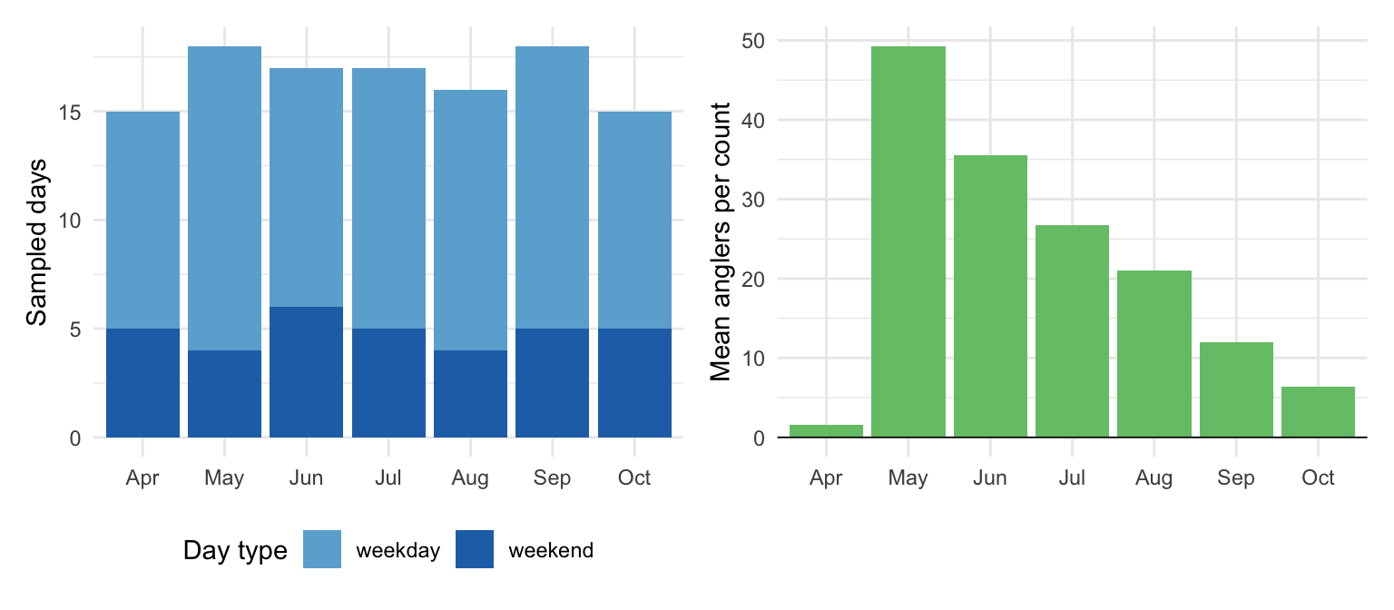
Sampling was distributed across the seven-month open-water season (April through October), with approximately two to six survey days per week in each stratum.
Figure 30.1: Monthly sampling effort and mean instantaneous angler count at Harlan Reservoir, 2022. Left: number of sampled days per month by stratum. Right: mean total anglers per count by month. The low April count reflects survey startup; May peaks near 50 anglers per count as the season opens.
Angler pressure rises sharply from April (1.9 mean anglers per count) to a May peak of 55.2 anglers per count, then declines steadily through October (7.3 mean anglers per count). The low April count reflects survey startup — sampling began April 2 and the reservoir had not yet reached peak fishing pressure.
Angler composition
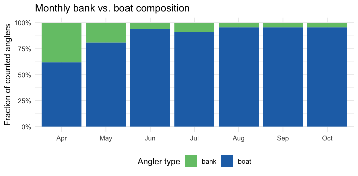
Harlan Reservoir is overwhelmingly boat-fished. Instantaneous counts record 90.9% boat anglers across all count events — consistent with a deep-water reservoir where White Bass and Walleye are most accessible from a vessel.
Figure 30.2: Monthly angler composition at Harlan Reservoir, 2022, from instantaneous count records. Boat anglers (blue) dominate throughout the open-water season. The bank-angling contingent is small but present in all months, concentrated near the shoreline access adjacent to the boat ramp.
The access-point interview composition differs from the count composition. Counts show 90.9% boat anglers, but interviews split 322 boat (53.7%) and 278 bank (46.3%). Bank anglers exit through the same access point as boat anglers — they park and walk rather than launching a trailer — making them proportionally easier to contact at the ramp than their share of the on-water count would suggest. This difference is important context for angler-type CPUE comparisons: the design-based estimator uses counts for effort expansion and interviews for rates, so the asymmetry does not bias either quantity. It does, however, mean that bank-angler CPUE is estimated from a sample that overrepresents that group relative to their presence on the water.
30.3 Building the design object
The Harlan pipeline follows the same four-step assembly used throughout Part III and in the Cedar Lake case study (Section 29.10). Three elements differ from the Cedar Lake roving build:
Asymmetric shift lengths. Period 1 covers eight hours and Period 2 covers six. A named vector maps period labels to shift lengths before add_counts() converts instantaneous counts to angler-hours. Using a single constant shift length would mismatch effort by up to 25% within each period.
Two catch columns derived before joining. The catch table stores species-level records with a catch_type flag. Per-interview harvest and release totals must be computed with group_by(interview_id) and then joined to the interview table. Both columns — total_harvest and total_catch (harvest + release) — are required by add_interviews().
Access interview type. Setting interview_type = "access" routes estimate_catch_rate() to the ratio-of-means estimator. Access-point designs capture complete trips at day end; ROM is appropriate because each interview contributes a full trip record.
Code
# Period shift lengthsshift_hours
1 2
8 6
Code
# Sample of preprocessed count records for one sampled dayharlan_counts_effort |>filter(date ==as.Date("2022-07-15")) |>select(date, day_type, period, count_time, angler_count, shift_length)
The split into total_harvest and total_catch is what allows the estimation layer to produce separate HPUE (harvest per unit effort) and CPUE (catch per unit effort) from the same interview record.
Effort at Harlan comes from the same instantaneous count estimator used throughout Part IV: average within-period counts, scale by shift length, expand sampled-day effort to the full stratum. The asymmetric shift lengths ride alongside the counts in harlan_counts_effort and are applied by add_counts() through period_length_col, so the design’s count column is already in angler-hours when estimate_effort() reads it.
Code
eff_tot$estimates
# A tibble: 1 × 7
  estimate    se se_between se_within ci_lower ci_upper     n
     <dbl> <dbl>      <dbl>     <dbl>    <dbl>    <dbl> <int>
1   38969. 3182.      2697.     1441.   32667.   45270.   118
Harlan anglers logged an estimated 38,969 angler-hours during the 2022 open-water season (95% CI: 32,667–45,270). The effort CV is 8.2%, driven primarily by between-day variance (SE between = 2697 vs SE within = 1441) — the dominant pattern for reservoir access-point surveys where daily boat-ramp traffic varies substantially with weather and day of week.
eff_strat$estimates |>ggplot(aes(estimate, fct_rev(day_type))) +geom_errorbarh(aes(xmin = ci_lower, xmax = ci_upper),height =0.15, linewidth =0.8) +geom_point(size =3, shape =21, fill ="#6baed6") +scale_x_continuous(labels = scales::comma) +labs(x ="Estimated effort (angler-hours)", y =NULL,title ="Season effort by day type") +theme_minimal(base_size =11)
Warning: `geom_errorbarh()` was deprecated in ggplot2 4.0.0.
ℹ Please use the `orientation` argument of `geom_errorbar()` instead.
`height` was translated to `width`.
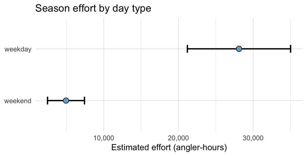
Figure 30.3: Season-total effort estimates by day-type stratum, Harlan Reservoir 2022. Points are ratio-of-means estimates; bars are 95% confidence intervals. Weekday effort is substantially higher than weekend effort, reflecting both the larger weekday frame and higher mean counts on weekdays.
Weekday effort (33,346 angler-hours) far exceeds weekend effort (5,623 angler-hours). The survey frame includes 150 weekday days versus 61 weekend days, so both the frame multiplier and higher mean weekday counts drive the difference. The non-overlapping confidence intervals confirm that the two strata genuinely differ and that stratification is adding information rather than noise to the effort estimate.
30.5 Catch, harvest, and release
Species catch composition
Harlan hosts eleven species in the catch record, spanning managed game fish, forage fish, and rough fish.
Code
harlan_catch |>group_by(species, catch_type) |>summarise(total =sum(n_fish), .groups ="drop") |>group_by(species) |>mutate(species_total =sum(total)) |>ungroup() |>filter(species_total >=10) |>mutate(species =fct_reorder(species, species_total)) |>ggplot(aes(total, species, fill = catch_type)) +geom_col(position ="stack") +scale_fill_manual(values =c(harvested ="#fd8d3c", released ="#74c476"),name ="Catch type") +scale_x_continuous(labels = scales::comma) +labs(x ="Fish recorded in interviews", y =NULL,title ="Interview catch composition by species (≥10 fish)") +theme_minimal(base_size =11) +theme(legend.position ="bottom")
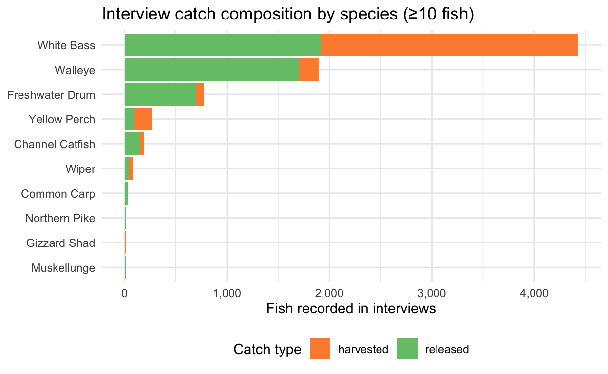
Figure 30.4: Total fish recorded in Harlan Reservoir interviews by species and catch type, showing only species with at least ten total fish. White Bass dominates in absolute numbers with a moderate harvest fraction. Walleye shows a pronounced release majority, consistent with the 381 mm size limit. Freshwater Drum are mostly released; Yellow Perch are mostly kept.
White Bass are kept at a moderate rate. Walleye show a high release fraction, driven by the 381 mm size limit — most fish encountered are sub-legal. Freshwater Drum are abundant but mostly released, reflecting low harvest interest despite no size restriction. Yellow Perch are kept at a high rate, consistent with their role as a preferred eating fish when encountered.
Season totals
Code
harv_tot$estimates
# A tibble: 1 × 5
  estimate    se ci_lower ci_upper     n
     <dbl> <dbl>    <dbl>    <dbl> <int>
1   22783. 2577.   17715.   27850.   390
Code
cat_tot$estimates
# A tibble: 1 × 5
  estimate    se ci_lower ci_upper     n
     <dbl> <dbl>    <dbl>    <dbl> <int>
1   58628. 5977.   46878.   70378.   390
Code
rel_tot$estimates
# A tibble: 1 × 5
  estimate    se ci_lower ci_upper     n
     <dbl> <dbl>    <dbl>    <dbl> <int>
1   35845. 4082.   27819.   43872.   390
Season harvest: 22,783 fish (95% CI: 17,715–27,850). Total catch: 58,628 fish (completed trips only, n = 390). Total release: 35,845 fish.
Harvest and release use all 600 interviews; total catch uses only the 390 completed trips. That difference explains why the harvest CV (11.3%) is lower than the total-catch CV (10.2%): harvest accesses the full interview sample, while total catch is constrained to completed trips where both elapsed time and fish-in-hand are known.
Weekday harvest (18,594 fish) is approximately 4.4 times weekend harvest (4,189 fish). The weekday dominance mirrors the effort pattern: more days in the frame, higher mean counts, and a larger angling population on weekdays during the open-water season at Harlan.
Walleye catch-and-release fishery
Walleye show 1699 releases against 200 harvested fish in the raw interview table — a 89.5% release fraction. The 381 mm size limit is the primary driver: most fish contacted fall below legal size and must be returned.
Of the 108 harvested Walleye with measured lengths, 74.1% met the 381 mm minimum. Mean length of harvested fish was 418 mm — well above the limit — indicating that anglers disproportionately retain the larger fish they encounter. That is the expected size-selective harvest pattern under a minimum-length regulation: sub-legal fish are released, legal fish are mostly kept, so the harvested sample skews toward large individuals.
30.6 CPUE and harvest rate
Access-point surveys use the ratio-of-means (ROM) estimator. Each completed trip contributes a fishing effort (hours_fished) and a catch total; the estimator divides the sum of catch across all trips by the sum of hours across all trips within a stratum. The ratio-of-means is appropriate here because access-point interviews capture full trips: start and end times are known, and the angler reports total catch for the entire trip.
Code
cpue_all$estimates
# A tibble: 1 × 5
  estimate     se ci_lower ci_upper     n
     <dbl>  <dbl>    <dbl>    <dbl> <int>
1     1.51 0.0928     1.32     1.69   390
Code
hpue_all$estimates
# A tibble: 1 × 5
  estimate     se ci_lower ci_upper     n
     <dbl>  <dbl>    <dbl>    <dbl> <int>
1    0.585 0.0464    0.495    0.676   390
Code
rpue_all$estimates
# A tibble: 1 × 5
  estimate     se ci_lower ci_upper     n
     <dbl>  <dbl>    <dbl>    <dbl> <int>
1    0.920 0.0733    0.776     1.06   390
Overall CPUE is 1.51 fish per angler-hour (95% CI: 1.32–1.69). The harvest rate is 0.59 fish per angler-hour and the release rate is 0.92 fish per angler-hour. Anglers released 61.1% of all fish caught — consistent with the high Walleye release fraction and moderate release rates for Freshwater Drum.
Weekday and weekend CPUE are nearly identical (1.48 and 1.64 fish per angler-hour, respectively) with overlapping confidence intervals. This is a common result in stratified creel surveys: stratification by day type is justified because effort differs between weekdays and weekends, but the catch rate experienced by individual anglers is roughly constant across the two groups. The stratum weights affect the effort total; they do not substantially affect the average rate.
CPUE by angler type
Boat and bank anglers at Harlan target different areas and species assemblages. Boat anglers access open water for White Bass and Walleye; bank anglers fish near the access-point shoreline where panfish and Channel Catfish are more common.
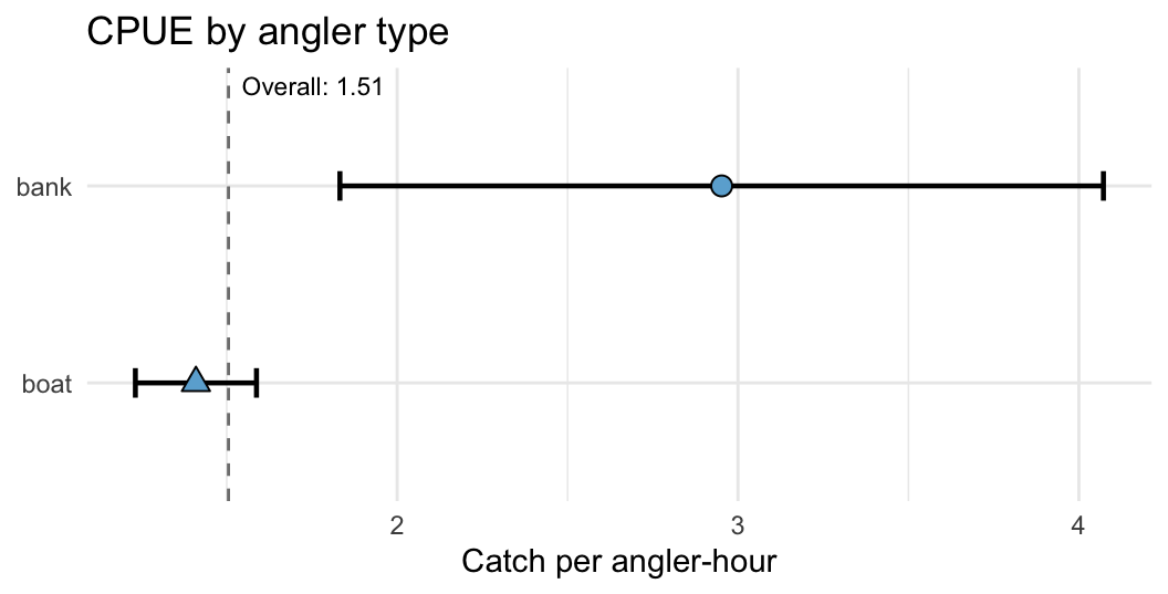
Figure 30.5: Catch per angler-hour by angler type at Harlan Reservoir, 2022. Points are ratio-of-means estimates from completed trips; bars are 95% confidence intervals. A dashed vertical line marks the overall CPUE. The bank sample is small (n < 80 completed trips), producing a wide confidence interval.
Bank anglers catch 2.95 fish per angler-hour versus 1.41 for boat anglers, but the bank-angler sample is small (71 completed trips). The wide bank confidence interval means the two point estimates are statistically indistinguishable at this sample size. Report the apparent contrast with the sample sizes shown here so readers can assess the uncertainty.
Species CPUE
With eleven species, the site-level CPUE conceals substantial species-level variation. estimate_catch_rate(by = species) produces a design-based estimate for each species using the same stratum weights.
Code
cpue_sp$estimates |>filter(estimate >0.01) |>select(species, estimate, se, ci_lower, ci_upper, n) |>arrange(desc(estimate))
White Bass (0.83 fish per angler-hour) and Walleye (0.39 fish per angler-hour) together account for most of the catchable rate. Freshwater Drum, Yellow Perch, Channel Catfish, and Wiper are present at measurable levels. The five species not shown — Crappie, Gizzard Shad, Common Carp, Northern Pike, and Muskellunge — have estimates below 0.01 fish per angler-hour; Gizzard Shad, Common Carp, and Muskellunge have confidence intervals that include zero. All five should be reported as incidental catches rather than targeted quantities.
30.7 Precision and diagnostics
A precision profile summarizes CV across all seven season-level estimates and identifies which quantities are solid enough for management use.
# A tibble: 7 × 3
  quantity      category    cv
  <chr>         <chr>    <dbl>
1 Effort        effort    8.16
2 Total harvest total    11.3
3 Total catch   total    10.2
4 Total release total    11.4
5 CPUE          rate      6.17
6 HPUE          rate      7.92
7 RPUE          rate      7.97
Code
cv_tbl |>mutate(quantity =fct_reorder(quantity, cv)) |>ggplot(aes(cv, quantity, fill = category)) +geom_col() +geom_vline(xintercept =20, linetype ="dashed", linewidth =0.6, color ="grey30") +scale_fill_manual(values =c(effort ="#6baed6", total ="#fd8d3c", rate ="#74c476"),name ="Estimate type" ) +labs(x ="CV (%)", y =NULL, title ="Precision profile") +theme_minimal(base_size =11) +theme(legend.position ="bottom")
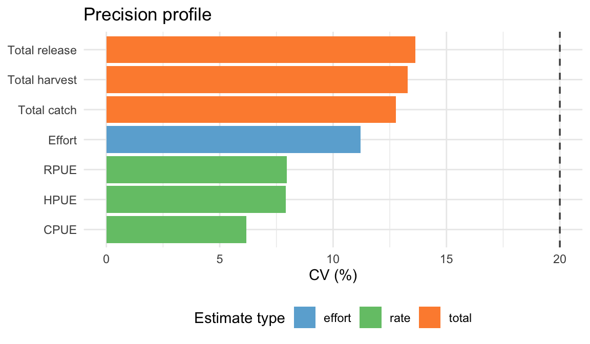
Figure 30.6: Coefficient of variation (%) for season-level estimates, Harlan Reservoir 2022. Dashed line at 20% marks the common management-grade precision threshold. Rate estimates are most precise because the ratio form stabilizes variance. Total release carries the highest CV, reflecting high per-trip variability in fish returned.
All seven estimates fall below the 20% management-grade threshold. CPUE is the most precise at 6.2% because the ROM estimator uses all 390 completed-trip observations and the ratio form stabilizes variance better than an expanded total. Effort CV at 8.2% is acceptable for a reservoir survey; the between-day component dominates because boat-ramp traffic fluctuates substantially with weather. Total release has the highest CV at 11.4%, reflecting higher per-trip variability in fish returned — occasional trips with large Walleye C&R events skew the release distribution. Total harvest (11.3%) and total catch (10.2%) are similar despite total catch using only the 390 completed trips.
The precision profile is most useful as a communication tool. Managers reading a creel report can quickly see which estimates carry enough precision to inform a regulation decision and which quantities — typically stratified sub-domains and rare species — carry wider uncertainty and should be interpreted cautiously.
30.8 Final report assembly
All estimates are assembled into a single reporting tibble, formatted for a non-technical audience, using the pattern from Section 26.3.
Code
report_summary <-bind_rows( eff_tot$estimates |>mutate(quantity ="Effort", unit ="angler-hours"), harv_tot$estimates |>mutate(quantity ="Total harvest", unit ="fish"), cat_tot$estimates |>mutate(quantity ="Total catch", unit ="fish"), rel_tot$estimates |>mutate(quantity ="Total release", unit ="fish"), cpue_all$estimates |>mutate(quantity ="CPUE", unit ="fish/hr"), hpue_all$estimates |>mutate(quantity ="HPUE", unit ="fish/hr"), rpue_all$estimates |>mutate(quantity ="RPUE", unit ="fish/hr")) |>select(quantity, unit, estimate, se, ci_lower, ci_upper)report_summary
# A tibble: 7 × 6
  quantity      unit          estimate        se  ci_lower  ci_upper
  <chr>         <chr>            <dbl>     <dbl>     <dbl>     <dbl>
1 Effort        angler-hours 38969.    3182.     32667.    45270.
2 Total harvest fish         22783.    2577.     17715.    27850.
3 Total catch   fish         58628.    5977.     46878.    70378.
4 Total release fish         35845.    4082.     27819.    43872.
5 CPUE          fish/hr          1.51     0.0928     1.32      1.69
6 HPUE          fish/hr          0.585    0.0464     0.495     0.676
7 RPUE          fish/hr          0.920    0.0733     0.776     1.06
Harlan Reservoir 2022 creel survey season estimates.
Quantity
Unit
Estimate
95% CI
CV
Effort
angler-hours
38,969
32,667–45,270
8.2%
Total harvest
fish
22,783
17,715–27,850
11.3%
Total catch
fish
58,628
46,878–70,378
10.2%
Total release
fish
35,845
27,819–43,872
11.4%
CPUE
fish/hr
1.51
1.32–1.69
6.2%
HPUE
fish/hr
0.59
0.49–0.68
7.9%
RPUE
fish/hr
0.92
0.78–1.06
8.0%
Inline narrative
Drawing directly from computed estimates, a one-page summary for managers reads:
NoteExample: manager one-page summary (excerpt)
Harlan Reservoir anglers logged an estimated 38,969 angler-hours during the 2022 open-water season (April 2–October 29). Total harvest was 22,783 fish (95% CI: 17,715–27,850 fish). Anglers caught 1.51 fish per angler-hour and harvested 0.59 fish per angler-hour across 116 sampled days and 600 interviews. Walleye showed a 89.5% release rate; 74.1% of harvested Walleye with measured lengths met the 381 mm minimum.
NoteExample: technical report footnote
Effort uses ratio-of-means with day-type stratification from instantaneous count data (two replicates per period; Period 1 = 8 hr, Period 2 = 6 hr). CPUE, HPUE, and RPUE use ratio-of-means from all completed trips (390 of 600 contacts; 65.0% completion rate). Total harvest and release use all 600 contacts; total catch uses the 390 completed trips only. Walleye compliance rate is based on 108 length-measured harvested Walleye (not all harvested Walleye were measured). Confidence intervals are 95% normal-approximation intervals from the design-based variance estimator. Domain: Harlan Reservoir, daylight hours, access-point at primary boat ramp, April 2–October 29, 2022.
30.9 Harlan versus Cedar Lake: a design contrast
The Cedar Lake case study (Section 29.10) analyzed that survey from the roving survey’s perspective. From Harlan’s access-point vantage point, the contrast in design choices and their downstream consequences is equally clear.
Design and estimate comparison between Harlan Reservoir and Cedar Lake case studies.
Feature
Harlan Reservoir
Cedar Lake
Survey period
April–October (7 months)
April–October (7 months)
Design type
Access-point (day-end)
Roving circuit (mid-trip)
Shift hours
8 hr / 6 hr (P1/P2)
6 hr / 6 hr (equal)
CPUE estimator
Ratio-of-means (ROM)
Mean-of-ratios (MOR)
Angler composition
91% boat (counts)
~91% bank
Interview completion
65% complete
~29% complete
Primary species
White Bass, Walleye
Bluegill, catfish, crappie
Season effort
~38,969 angler-hours
~12,200 angler-hours
CPUE
1.51 fish/hr
~2.09 fish/hr
Effort CV
8.2%
~5.3%
Harvest CV
11.3%
~6.4%
The estimator choice is the clearest difference. Harlan’s access-point design produces 65.0% completed trips; the ROM estimator is appropriate because every interview contributes a complete record. Cedar Lake’s roving design produces ~29% complete trips; the MOR estimator is required because most contacts are mid-trip observations.
Effort CV is actually higher at Harlan (8.2%) than at Cedar Lake (~5.3%) despite more sampled days. Harlan’s boat-ramp count record has higher between-day variance: daily angler counts swing sharply with weather and season on a large reservoir, while Cedar Lake’s shoreline walk-count is more stable on a smaller body of water. Survey design precision depends as much on the fishery’s natural variability as on the number of sampled days.
30.10 Takeaway
The Harlan Reservoir case study synthesizes the estimation chapters from Part IV into a single access-point pipeline. Three choices drive the analysis:
Access-point design → ratio-of-means. Day-end interviews at the boat ramp capture departing parties with complete trip records. ROM divides total catch by total hours across the full interview set — the right estimator when trips are observed in their entirety. Choosing MOR instead would require treating each interview as an instantaneous rate observation, which is not appropriate when hours fished and total catch are both complete.
Period-asymmetric shifts → encode shift lengths before estimation. A morning shift of eight hours and an afternoon shift of six hours require a named vector before counts are converted to angler-hours. Using a single constant would mismatch effort by up to 25% within each period and propagate that error into every downstream estimate scaled by effort.
Boat-dominant fishery → interpret angler-type CPUE with sample size. Boat anglers account for 90.9% of counted anglers but only 53.7% of interviews. The design-based estimator handles this correctly — counts drive effort expansion, interviews drive rates — but the bank-angler CPUE sub-domain is based on only 71 completed trips. Always report the n alongside the estimate so readers can assess the stability of sub-domain contrasts.
The season estimates — 38,969 angler-hours, 22,783 fish harvested, 1.51 fish per angler-hour — all meet the 20% CV threshold. For a seven-month access-point survey with asymmetric period lengths and a multi-species catch record, that represents a cost-effective characterization of a diverse reservoir fishery.
30.11 Reproducibility note
The Harlan Reservoir estimates in this chapter reproduce exactly given the same data files and package version:
Loading the saved design restores the full stratum structure, counts, interview data, and catch table in a single call, ready for any subsequent estimate_*() call.