24Biological Data from Interviews: Length Distributions and Size Compliance
Author
Christopher Chizinski
Keywords
creel survey, fisheries, design-based inference, R, tidycreel, Quarto
Section 21.1 through Section 23.2 estimated how many fish were caught, kept, and released. Those are count quantities — numbers that answer “how many?” But many management decisions require a different kind of question: “what size?” A walleye harvest total of 4,000 fish means something very different depending on whether those fish averaged 300 mm or 500 mm. A size-limit regulation can only be evaluated if the agency knows how many harvested fish were actually legal-sized. A population assessment comparing creel data to electrofishing samples requires both surveys to speak the same biological language.
Creel surveys have always produced biological data alongside catch and effort data. Interview clerks routinely measure harvested fish, record lengths of fish returned to the water, and sometimes collect scale or fin ray samples for aging. That information lives in a separate table — one row per fish measured, linked back to the interview by a common identifier — and it requires a distinct estimation workflow. This chapter covers that workflow from data preparation through design-weighted length-frequency estimation to regulatory compliance analysis.
24.1 Why biological data require their own estimator
The intuition behind catch-rate estimation is straightforward: a ratio of means applied across a weighted interview sample. Length estimation has the same logical foundation but a subtle complication. Fish are subsampled within interviews. Not every harvested fish is measured — a party of six anglers returning with a mixed bag of 18 white bass and 4 walleye will often have lengths recorded for only a portion of each species. The clerk may measure all walleye but only a random five of the white bass, or measure no fish at all if the party is rushed.
This two-stage structure — sampling days within a survey season, then sampling fish within interviews — means that naive pooling of all measured lengths is not a valid population-level estimate. The sample of fish you measure is not a simple random sample of all fish harvested at Harlan Reservoir during the season; it is a convenience subsample embedded in a probability sample of interviews. To recover a population-weighted distribution, you must propagate interview-level uncertainty through the survey design, exactly as you do for effort and catch totals (Pollock et al. 1994).
tidycreel provides two functions for this workflow. summarize_length_freq() produces unweighted sample frequencies — the raw fraction of measured fish in each size bin, useful for exploratory work and for checking data structure. est_length_distribution() applies the interview survey weights from the creel_design object to produce design-based estimates of length-frequency with standard errors and confidence intervals. Both require the same data preparation step: attaching a length table to the design with add_lengths().
24.2 The length data structure
Length data at Harlan Reservoir are stored in harlan_lengths, a table with one row per measured fish (for individual measurements) or per occupied bin (for binned release records).
Three species with length records: White Bass (the most abundant harvest at Harlan), Walleye (a regulated species with a 381-mm minimum size limit), and Channel Catfish. Walleye release records use a binned format — the clerk recorded how many released fish fell into each 50-mm bin (e.g., "300-350", "350-400") rather than measuring each individual. This is common practice for large numbers of released fish: counting by length class at streamside is faster than individual measurement and retains the information needed for compliance and recruitment analysis. Individual harvest lengths are stored as a numeric value in the length column, with count = NA; binned release records carry the bin label as a character string and a non-missing fish count in count.
Code
# Individual harvest records: length is numeric, count is NAharlan_lengths |>filter(length_type =="harvest") |>slice_head(n =5)
  interview_id    species length length_type count
1           97 White Bass    325     harvest    NA
2           97 White Bass    239     harvest    NA
3           97 White Bass    273     harvest    NA
4           97 White Bass    299     harvest    NA
5           97 White Bass    273     harvest    NA
Code
# Binned release records: length is a bin label, count is fish per binharlan_lengths |>filter(length_type =="release") |>slice_head(n =8)
The column names and mixed types in length (numeric for harvest, character for release bins) are handled internally by add_lengths() through the release_format argument. Setting release_format = "binned" tells the function that release rows carry count totals per bin label rather than individual measurements.
24.3 Building the design with length data
The length table attaches to the creel design after add_interviews(). As in Section 22.3, the interview table must carry species-level catch summaries as separate columns before being passed to add_interviews().
Printing design_bio confirms that the $catch and $lengths slots are now populated. The design object carries the length column mapping internally — species, length, length_type, and count are registered at attachment time so that summarize_length_freq() and est_length_distribution() can locate the right columns without requiring the analyst to re-specify them.
add_catch() attaches the species-level catch records, and it is not optional here. Lengths are measured on a subsample of the harvest, so a bin total means nothing until it is scaled to a reported catch total — and for a per-species distribution that total has to be that species’ harvest, not the all-species figure. The interview-level harvested column supplied to add_interviews() above pools every species together, so on its own it cannot scale a Walleye distribution. est_length_distribution(by = species) refuses rather than silently scaling Walleye lengths by a harvest that includes White Bass and Channel Catfish.
add_lengths() validates that every interview ID in harlan_lengths exists in design_bio$interviews — interviews with no length records are valid (not every angler’s catch is measured), but lengths cannot appear for interviews that are absent from the design. The function registers the column mapping internally so subsequent calls to summarize_length_freq() and est_length_distribution() know which column holds lengths and which identifies the interview link.
24.4 Raw length-frequency distributions
The first look at biological data should always be the unweighted sample frequencies. summarize_length_freq() returns the raw count of measured fish per bin, the percentage within each species, and a cumulative percentage — the same numbers you would compute from a flat spreadsheet. This is fast and useful for detecting data entry errors (lengths outside plausible biological range), checking bin coverage, and building a sense of the data before applying the survey weights.
Code
lf_raw <-summarize_length_freq(design_bio, type ="harvest", by = species, bin_width =25)lf_raw
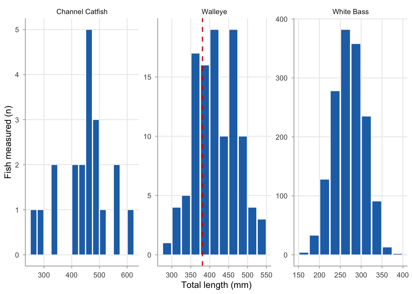
Figure 24.1 shows these distributions side by side. The three species have strikingly different shapes: White Bass form a compact, near-symmetric distribution around 265 mm; Walleye are spread broadly from about 275 mm to 550 mm with a mode near 425 mm and a visible left tail below the 381-mm size limit; Channel Catfish span the widest range, 250–625 mm, reflecting the wide age and size structure typical of catfish populations.
Figure 24.1: Sample length-frequency distributions for three species at Harlan Reservoir. Bars show raw counts of individually measured harvest fish in 25-mm bins. Vertical dashed line on the Walleye panel marks the Nebraska 381-mm minimum size limit. White Bass have the tightest distribution; Channel Catfish the widest. Distributions are unweighted sample frequencies, not population-weighted estimates.
The raw counts are informative but not directly interpretable as population estimates. An interview from a busy summer weekend with 40 measured walleye gets the same weight as a quiet Tuesday interview with 3 measured fish, even though the weekday interview represents a stratum sampled at a different rate. The weighted estimator corrects for this.
24.5 Design-weighted length distributions
est_length_distribution() produces a pressure-weighted length-frequency estimate: each interview’s length contribution is scaled by the survey weights in the creel_design object, so the resulting distribution reflects the frequency at which different size fish were harvested across the full survey season, not just the frequency with which they appeared in the sampled interviews.
Warning: ! Length totals were rescaled onto the reported catch.
ℹ Measured fish (weighted): 1652; reported: 2741 -- a factor of 1.66.
ℹ estimate, se and the confidence bounds describe the REPORTED catch, estimated
  from the measured subsample. Shares (percent) are unaffected.
The warning is expected and worth reading rather than suppressing. It reports the scaling factor applied — here the weighted measured fish are rescaled up to the reported harvest — and states plainly which columns it affects: estimate, se and the confidence bounds describe the reported catch, estimated from the measured subsample, while the percentage columns are shares and so are untouched. A length distribution that skipped this step would describe only the fish that happened to be measured.
Each row now carries a se, ci_lower, and ci_upper alongside the point estimate. The standard error propagates interview-level variation through the stratified design — bins that appeared inconsistently across sampled interviews have wider intervals, reflecting genuine uncertainty about how common that size class was in the harvested population.
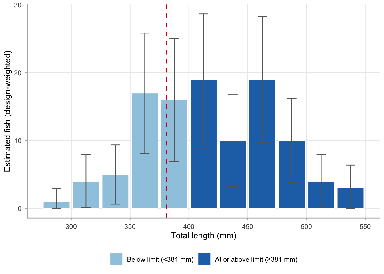
Figure 24.2 shows the weighted Walleye distribution. Several features stand out that are not obvious from the raw count histogram: the confidence intervals are widest in the central bins (400–450 mm) where interview-to-interview variation in the count of fish of this size is largest, and narrowest at the tails where either fish are consistently absent or consistently few. The dashed line marks the Nebraska minimum size limit of 381 mm (15 in); the large majority of the estimated harvest falls above this threshold.
Figure 24.2: Design-weighted harvest length distribution for Walleye at Harlan Reservoir. Point estimates (bars) reflect interview-survey-weighted proportions of harvested fish by 25-mm length class. Error bars are 95% confidence intervals. Dashed red line marks the 381-mm (15-in) Nebraska minimum size limit. Bins entirely below the size limit appear in a lighter shade to highlight the sublegal fraction.
The confidence intervals in Figure 24.2 are wide — a natural consequence of the modest number of interviews with length records and the across-interview variability in fish size. This uncertainty should accompany any regulatory reporting that relies on these estimates.
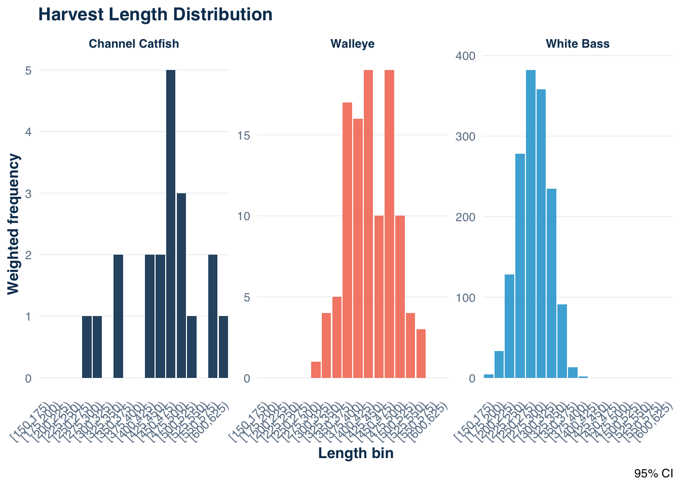
The creel_length_distribution object has an autoplot() method that renders a quick faceted bar chart with error bars across all grouping levels — useful for exploring all three species simultaneously before deciding which to examine more closely.
Code
ggplot2::autoplot(lf_weighted, theme ="creel")
Figure 24.3: Design-weighted harvest length distributions for all three species at Harlan Reservoir, produced by ggplot2::autoplot(). Error bars show 95% confidence intervals. The faceted layout reveals that White Bass have the narrowest distribution, Channel Catfish the widest, and Walleye straddle the 381-mm size limit. Use this plot for rapid exploration; Figure 24.2 provides the annotated version for reporting.
24.6 Interview coverage and subsampling intensity
Before relying on a length distribution estimate, it is worth asking how many interviews contributed length records and whether that subsample is spread across the survey schedule. A length distribution estimated from twelve interviews — even if those interviews covered many fish — carries more uncertainty than one supported by sixty interviews spread across weekdays and weekends throughout the season.
Length records were collected from approximately 27% of interviews in each stratum. Coverage that is roughly equal across strata — as it is here — means that subsampling is not systematically biasing the length distribution toward one day type. If weekday interviews had dramatically lower coverage than weekend interviews, the estimated distribution would lean toward the weekend fish composition, which could differ in size structure if fishing pressure and selectivity differ by day type.
The subsample rate also has a direct effect on precision. More measured fish within an interview reduces within-interview variability in the length column; more interviews with any length records reduces between-interview variability. For a fixed field budget, measuring a few fish across more interviews is more efficient than measuring many fish in fewer interviews, because between-interview variance dominates total variance in stratified survey estimators — a pattern visible in the variance decomposition for effort in Section 25.1.
est_length_distribution() offers three variance estimation methods (set via the variance argument): "taylor" (default, delta-method), "bootstrap", and "jackknife". For small biological subsamples — fewer than twenty to thirty interviews with length records — the bootstrap or jackknife approaches often give more conservative and reliable uncertainty bounds than the delta-method approximation.
24.7 Released fish: binned length distributions
The type argument to est_length_distribution() controls which fish are included. Setting type = "release" pulls the binned Walleye release records and produces a distribution of the returned fish. Because released fish were binned in 50-mm intervals rather than measured individually, a wider bin_width is appropriate.
Warning: ! Length totals were rescaled onto the reported catch.
ℹ Measured fish (weighted): 498; reported: 1699 -- a factor of 3.41.
ℹ estimate, se and the confidence bounds describe the REPORTED catch, estimated
  from the measured subsample. Shares (percent) are unaffected.
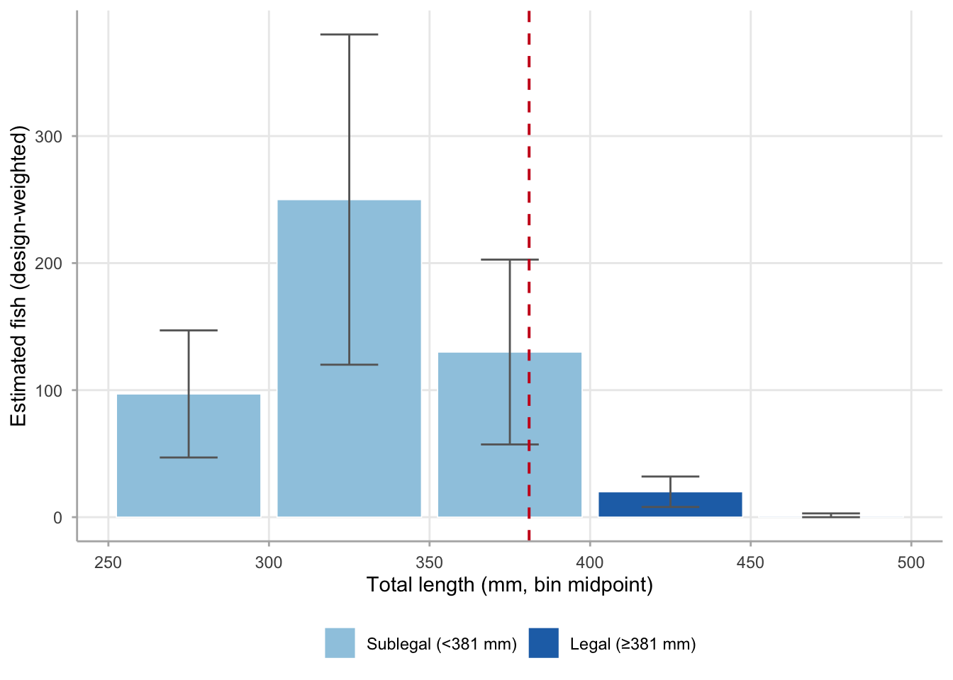
The release distribution tells a complementary story to the harvest distribution. Whereas harvested Walleye were concentrated above 375 mm, released fish are concentrated below 381 mm — almost 96% of estimated released Walleye fell below the size limit (Figure 24.4). This is the expected pattern under a minimum size regulation: anglers keep legal fish and return sublegal fish.
Figure 24.4: Design-weighted length distribution of released Walleye at Harlan Reservoir, binned at 50-mm intervals. The 381-mm size limit (dashed red line) cleanly separates the release distribution from the harvest distribution in Figure 24.2: nearly all released fish were sublegal, consistent with angler compliance with the minimum size regulation.
The complementarity of harvest and release distributions is itself a data quality diagnostic. If a substantial fraction of estimated released fish exceeded the size limit, or if harvested fish frequently appeared below it, that would raise questions about either reporting accuracy or measurement error — both worth investigating before the data enter a regulatory assessment.
24.8 Weighted mean length from the estimated distribution
est_mean_length() computes the design-weighted mean length directly from a creel_length_distribution object, using the ratio estimator \bar{L} = \sum_h L_h \hat{N}_h / \hat{N} with delta-method standard error. Bin midpoints serve as representative lengths within each class.
# A tibble: 3 × 3
  species         mean_length_raw_mm     n
  <chr>                        <dbl> <int>
1 Channel Catfish               451.    20
2 Walleye                       418.   108
3 White Bass                    270.  1524
When the two means agree closely, the interview subsampling was roughly self-weighting with respect to mean fish size — interviews that measured more fish did not systematically measure larger or smaller fish than interviews that measured fewer. A discrepancy between the two means signals a correlation between interview-level subsampling intensity and fish size, which can arise, for example, if clerks measured more fish during periods when anglers were catching larger individuals (peak season, favorable conditions). In that case, the design-weighted mean from est_mean_length() is the more defensible estimate, because it propagates survey weights through the ratio estimator rather than treating all measured fish as equally representative. For Harlan Walleye, the two means should be close, consistent with the balanced subsampling coverage shown in the previous section.
24.9 Size-limit compliance analysis
est_compliance() estimates the design-weighted compliance proportion directly from a creel_length_distribution object. Bins whose lower bound is at or above the minimum legal length are classified as legal; bins that straddle the threshold are classified as illegal (a conservative rule that avoids overstating compliance when fish cluster near the limit). The estimator is the ratio of estimated legal fish to estimated total fish, with delta-method standard error.
60.2% of estimated harvested Walleye at Harlan Reservoir met or exceeded the 381-mm size limit (95% CI: 52.2–68.2%). This is the design-weighted estimate: it accounts for the stratified survey structure rather than treating all measured fish as a simple random sample.
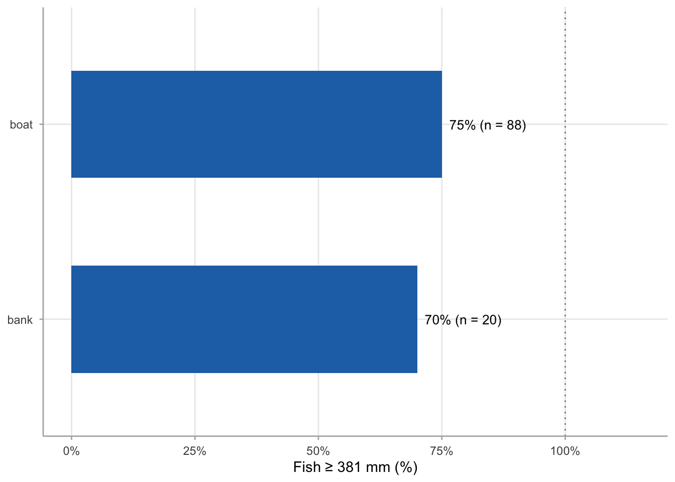
Figure 24.5 breaks compliance down by angler type using the raw length sample — a decomposition that can reveal whether boat and bank anglers differ in the size composition of their harvest. Access differences between angler types often translate into size-structure differences because boat anglers can reach deeper structures where larger fish concentrate.
Figure 24.5: Walleye harvest size compliance by angler type at Harlan Reservoir. Bars show the percentage of individually measured harvested Walleye that met or exceeded the 381-mm (15-in) minimum size limit. Labels to the right of each bar show the percentage and the sample size of measured fish. Both angler types show high compliance, with boat anglers harvesting a modestly larger fraction of legal-size fish.
Boat anglers show marginally higher compliance than bank anglers, consistent with their ability to target deeper water where larger fish concentrate. The difference is not statistically tested here — a formal design-weighted contrast would require a separate est_length_distribution(design_bio, ..., by = angler_type) call followed by est_compliance() per angler type. The overall design-weighted estimate produced above is the more defensible number for regulatory reporting.
24.10 Estimating biomass from the length distribution
est_biomass() converts a design-weighted length-frequency distribution into a total biomass estimate using the allometric length-weight equation W = a \cdot L^b. It applies the relationship at each bin midpoint to approximate the distribution-weighted mean weight and propagates uncertainty via the delta method, yielding a biomass estimate with a confidence interval.
For Walleye, a commonly used length-weight relationship takes the form W = a \cdot L^b where W is weight in grams and L is total length in mm. Example parameters (a = 0.0000106, b = 3.093) are illustrative; programs should fit species- and water-body-specific coefficients from their own biological sampling data.
Code
# Length-weight parameters for Walleye (W in grams, L in mm)a <-0.0000106b <-3.093lf_walleye_harvest <- lf_weighted |>filter(species =="Walleye")biomass_walleye <-est_biomass(lf_walleye_harvest, a = a, b = b)biomass_walleye
This calculation uses the bin midpoint as a representative length for all fish in that class — an approximation that is accurate when bins are narrow relative to the range of the distribution, which is the case with 25-mm bins. Unlike a manual bin-by-bin calculation, est_biomass() propagates uncertainty from the estimated fish counts through the length-weight transformation via the delta method, so the result includes a 95% confidence interval on total biomass.
24.11tidycreel support
tidycreel supports the full biological estimation workflow through ten functions:
Function
Purpose
add_lengths()
Attach a length table to a creel_design; validates interview IDs and column types; handles individual and binned formats
add_ages()
Attach an age table (scale, fin ray, or otolith) to a creel_design; mirrors add_lengths()
summarize_length_freq()
Unweighted sample frequency by bin and species; for exploration and QA
est_length_distribution()
Design-weighted length-frequency with SE and 95% CI; produces creel_length_distribution object
autoplot()
Default plot method for creel_length_distribution objects; quick visualization without manual ggplot construction
est_mean_length()
Design-weighted mean length from a creel_length_distribution object; ratio estimator with delta-method SE
est_compliance()
Design-weighted size-limit compliance proportion; bins at or above min_length classified as legal
est_biomass()
Total biomass from a creel_length_distribution object via W = aL^b; delta-method CI
est_age_distribution()
Design-weighted age-frequency with SE and 95% CI from an add_ages() object; produces creel_age_distribution
est_mean_age()
Design-weighted mean age from a creel_age_distribution object; ratio estimator with delta-method SE
The workflow for length data is: add_lengths() → est_length_distribution() → est_mean_length() / est_compliance() / est_biomass(). The workflow for age data mirrors it exactly: add_ages() → est_age_distribution() → est_mean_age(). The following example uses the tidycreel package’s built-in example_ages dataset; field programs that collect otolith or scale ages follow the same pipeline with their own age tables.
Code
data(example_calendar)data(example_interviews)data(example_ages)data(example_catch)design_age <-creel_design(example_calendar, date = date, strata = day_type) |>add_interviews(example_interviews,catch = catch_total, effort = hours_fished, harvest = catch_kept,trip_status = trip_status ) |># Species-level catch, for the same reason as `design_bio` above: an age# distribution grouped by species must be scaled to that species' harvest.add_catch(example_catch,catch_uid = interview_id,interview_uid = interview_id,species = species,count = count,catch_type = catch_type ) |>add_ages(example_ages,age_uid = interview_id,interview_uid = interview_id,species = species,age = age,age_type = age_type )
Warning: ! No `n_anglers` provided — assuming 1 angler per interview.
ℹ Pass `n_anglers = <column>` to use actual party sizes for angler-hour
  normalization.
ℹ If the interviews really are one angler each, pass `n_anglers = 1` to state
  that and silence this warning.
ad <-est_age_distribution(design_age, by = species, type ="harvest")
Warning: ! Age totals were rescaled onto the reported catch.
ℹ Measured fish (weighted): 12; reported: 59 -- a factor of 4.92.
ℹ estimate, se and the confidence bounds describe the REPORTED catch, estimated
  from the measured subsample. Shares (percent) are unaffected.
The creel_age_distribution object returned by est_age_distribution() has the same structure as creel_length_distribution: one row per age class (with grouping columns when by is supplied), plus estimate, se, ci_lower, ci_upper, percent, and cumulative_percent. est_mean_age() returns the ratio-estimated mean age and its delta-method standard error.
One gap remains without automated support: exploitation rate by size class, which requires combining creel harvest estimates with population abundance from an independent survey (electrofishing or gill-netting). That calculation is not automated because the abundance denominator comes from outside tidycreel’s scope. The key principle for analysts who need it is the same as for the functions above: express the biological quantity as an interview-level observation, attach it to the design, and let the stratified estimator propagate uncertainty.
24.12 QA check: combined catch distribution
A useful final check before any biological results leave the analyst’s desk is to compare the combined catch distribution (type = "catch", which includes harvest and release together) against the harvest-only and release-only distributions. The combined total should equal the sum of the two components, and the size structure should fall between them — more large fish than the release distribution, fewer than the harvest distribution alone.
Code
summarize_length_freq(design_bio, type ="catch", by = species, bin_width =25) |>filter(species =="Walleye") |>select(species, length_bin, N, percent, cumulative_percent)
The combined Walleye distribution is distinctly bimodal: a left mode from sublegal released fish concentrated below 381 mm, and a right mode from legal harvested fish concentrated above 381 mm. Neither component alone shows this bimodality. This is the full size structure of Walleye contacted at Harlan Reservoir — the population the fishery is drawing on — and it confirms that the regulation is achieving its intended selectivity: anglers are retaining fish that have grown past the minimum length while returning the smaller cohort to continue growing.
If the combined distribution were unimodal and concentrated above the size limit, it would suggest either that sublegal fish were present but not being reported as released, or that the fish population lacks a strong sublegal cohort — both worth documenting. If it were concentrated entirely below the limit, it would indicate a recruitment failure or harvest of sublegal fish.
24.13 Takeaway
Biological data from creel interviews require a two-stage estimation approach: fish are subsampled within interviews, which are themselves sampled as part of a stratified survey. Treating measured fish as a simple random sample ignores the survey structure and produces length distributions that reflect sampler convenience rather than angler harvest. add_lengths() attaches the length table to the creel_design object so that est_length_distribution() can apply interview-level survey weights to recover a design-based estimate of the harvested size composition.
At Harlan Reservoir, the design-weighted Walleye harvest compliance estimate was 60.2% (95% CI: 52.2–68.2%). The complementary release distribution — concentrated below the size limit — confirms that anglers at Harlan were returning sublegal fish rather than harvesting them. Together, these two distributions provide the regulatory evidence base that effort and catch totals alone cannot supply.
Section 25.1 covers precision diagnostics for effort and catch-rate estimates; the same CV-based framework applies to length distribution estimates, where the coefficient of variation on key bins (the sublegal fraction, the modal bin) is the natural precision target for planning biological subsampling intensity in future seasons.
The biological estimation workflow adds one or two steps to the standard pipeline — add_lengths() for size data, add_ages() for age data, each placed after add_interviews() — and unlocks the full suite of biological summary functions. The complete sequence from linked tables to design-weighted compliance, mean length, biomass, age distribution, and mean age requires no additional packages beyond tidycreel and tidyverse.
Pollock, K. H., C. M. Jones, and T. L. Brown. 1994. Angler survey methods and their applications in fisheries management. American Fisheries Society, Bethesda, Maryland.