creel survey, fisheries, design-based inference, R, tidycreel, Quarto
Every creel estimate traces back to a field form. The variables your technicians record determine which estimators you can run, which domains you can analyze, and which management questions you can answer. A perfectly designed sampling schedule and a well-executed field season still cannot produce harvest-by-species estimates if the interview form combined harvest and release into a single “catch” tally. This chapter describes the instrument design decisions that shape the downstream analysis workflow in tidycreel.
This is a “before the data exist” chapter. Survey design determines when and where data are collected; instrument design determines what those data contain. Both are equally binding. Survey design gaps can sometimes be partially corrected in analysis — for example, by re-weighting strata or adjusting for unequal probability of selection. Instrument design gaps cannot: a column that was never on the form cannot be recovered after the season ends.
The analogy to tidy data is direct: an underspecified creel interview form constrains which estimation pathways are available, just as an untidy data structure constrains which analytical methods apply. Getting the form right is not a clerical concern — it is a statistical design decision.
16.1 The tidycreel schema as interview blueprint
tidycreel is built around an explicit data contract expressed through creel_schema(). Every column the package touches — in interviews, counts, catch, and lengths tables — has a named slot in the schema. Creating a schema for your survey is the natural first step in translating a paper or digital interview form into an R-compatible data structure.
The Harlan schema maps the 2022 column names to their canonical tidycreel slots:
The schema maps canonical tidycreel variable names (left side) to the actual column names in your data (right side). Every non-NULL slot corresponds to a question on your interview or count form. A NULL slot means that variable will not be available for estimation — and that is a deliberate, documented decision, not an oversight.
Schema fields grouped by form
Table 16.1 groups each schema slot by the form it belongs on and the estimation it enables.
Table 16.1: Tidycreel schema fields grouped by data source. Each field corresponds to a question on the interview or count form, or a column in the catch table. Missing fields (NULL in schema) remove specific estimation capabilities.
Form
Schema slot
Canonical column
Enables
Interview
interview_uid_col
interview_id
Record linkage, deduplication
Interview
date_col
date
All temporal stratification
Interview
effort_col
hours_fished
CPUE, trip-duration CPUE
Interview
trip_status_col
trip_status
Complete/incomplete split for estimator selection
Interview
n_anglers_col
n_anglers
Party-size expansion
Interview
angler_type_col
angler_type
Bank vs. boat domain estimates
Interview
angler_method_col
angler_method
Gear-specific catch rates
Interview
species_sought_col
(not collected)
Target species filtering
Interview
refused_col
(not collected)
Nonresponse bias assessment
Count
bank_anglers_col
bank_anglers
Effort expansion for bank anglers
Count
angler_boats_col
angler_boats
Effort expansion for boat anglers
Count
count_col
bank_anglers
Total instantaneous count
Catch (linked)
catch_uid_col
interview_id
Species-level catch linkage
Catch (linked)
species_col
species
Species-specific harvest/CPUE
Catch (linked)
catch_count_col
n_fish
Fish counts per species per type
Catch (linked)
catch_type_col
catch_type
Harvest vs. release distinction
Two slots — species_sought_col and refused_col — show “(not collected)” for the Harlan 2022 survey. Those gaps close off target-species filtering and nonresponse assessment for that dataset. The sections below describe each form in turn and explain which capabilities depend on which fields.
16.2 Interview form design
Data structure: what the interview table looks like
The interview table is a flat, one-row-per-interview data frame. Each row represents one contacted party on one sampling day. The columns fall into two categories: administrative fields (date, stratum, location) and measurement fields (effort, angler count, trip status). Catch is not in the interview table — it lives in a separate linked catch table, joined on interview_id.
# A tibble: 6 × 9
  date       day_type interview_id party_id  n_anglers angler_type angler_method
  <date>     <chr>           <int> <chr>         <dbl> <chr>       <chr>
1 2022-09-01 weekday             1 6efcab06…         4 boat        Rod and Reel
2 2022-09-01 weekday             2 d19b214a…         3 bank        Rod and Reel
3 2022-09-01 weekday             3 0093195d…         3 bank        Rod and Reel
4 2022-09-01 weekday             4 e929b06d…         2 boat        Rod and Reel
5 2022-09-01 weekday             5 0c740e97…         2 boat        Rod and Reel
6 2022-09-01 weekday             6 247f59b7…         2 boat        Rod and Reel
# ℹ 2 more variables: hours_fished <dbl>, trip_status <chr>
The separation between the interview table and the catch table is a deliberate design choice, not a database artifact. It mirrors the physical data collection workflow: the interview form captures party-level metadata, while the catch recording (species, count, fate) happens per-fish or per-species in a separate tally. Section 18.1 explains why premature flattening of this structure — joining catch into the interview row — causes problems for estimation.
Core fields
Every creel interview, regardless of survey type, needs six pieces of information:
Date — to assign interviews to the correct stratum
Interview identifier — to link interviews to catch records
Angler count (n_anglers) — the number of anglers in the party
Effort (hours_fished) — time fished by the party at interview time
Trip status (trip_status) — whether the trip is complete or ongoing
Species-level catch — recorded in a linked catch table, not as an interview-level total
These six fields are the minimum viable interview. Without any one of them, a specific estimator fails: no date means no temporal stratification, no trip status means the estimator cannot distinguish MOR from ROM, no catch means no harvest or CPUE.
Recording catch: harvest, release, and total
The single most consequential form design decision is how catch is recorded. tidycreel uses a long-format linked catch table where each row is one species × catch_type combination. The catch_type column distinguishes three fates:
"harvested" — kept fish
"released" — released fish
"caught" (or "total") — all fish, without fate distinction
Recording all three types enables estimate_total_harvest(), estimate_total_catch(), and estimate_total_release() independently. Recording only totals forecloses harvest and release estimation — a serious constraint for regulation compliance work, where the harvest rate is often the primary output.
The catch table uses one row per species per catch type per interview. An interview that yields 32 harvested and 11 released White Bass produces two rows — one for each fate. This long format supports any combination of species, catch types, and interview records without restructuring the table.
Code
harlan_catch |>head(6)
# A tibble: 6 × 4
  interview_id species         catch_type n_fish
         <int> <chr>           <chr>       <int>
1            1 White Bass      released       11
2            1 White Bass      harvested      32
3            1 Yellow Perch    released        1
4            1 Walleye         released        0
5            4 White Bass      harvested       9
6            4 Freshwater Drum released        3
Code
harlan_catch |>count(catch_type) |>mutate(pct =round(100* n /sum(n), 1))
# A tibble: 2 × 3
  catch_type     n   pct
  <chr>      <int> <dbl>
1 harvested    430  43.6
2 released     557  56.4
Harlan records both "harvested" and "released" rows — enabling harvest-rate and release-rate estimation throughout Part IV.
Trip completeness: access-point vs. roving
The trip status field has different implications depending on survey design:
Access-point interviews collect mostly complete trips (anglers departing the access point). The estimator multiplies mean catch by total effort without a bias-correction term.
Roving interviews interrupt trips mid-day. The mean-of-ratios (MOR) estimator uses all trips regardless of status; the ratio-of-means (ROM) uses only complete trips. The use_trips argument in estimate_catch_rate() selects the estimator, but only if trip status was recorded.
A form that records trip status as a binary flag ("complete" / "incomplete") gives full flexibility. A form that omits trip status forces the analyst to assume all trips are complete — an assumption that inflates CPUE in roving surveys (Pollock et al. 1994).
Effort: what anglers can tell you
The hours_fished variable is the effort denominator for CPUE. For complete trips, it is the actual fishing duration for the party. For incomplete trips in roving surveys, it is the time fished up to the interview moment. Both values are meaningful; the estimator handles the difference.
Anglers in some fisheries fish in shifts or use multiple methods sequentially. The party-level hours_fished field is sufficient for most applications. If individual-level effort is needed — for example, to compute person-hours when party members start and stop at different times — you would need additional fields (trip_start_col, interview_time_col).
16.3 Effort count form design
Data structure: what the count table looks like
The count table records one row per count event. For an instantaneous design with two counts per sampling day, each survey date appears twice. Each row captures the counts at a specific time point: bank_anglers, angler_boats, and boat_anglers (derived from angler_boats × mean(anglers/boat) from interview data).
The count table links to the interview table by date and day_type. It does not link at the interview level — counts are whole-day estimates, while interviews are party-level.
The count form runs independently of the interview form. Enumerators count anglers at a fixed moment (instantaneous design) or progressively along a route (bus route design). The two fields that matter most are bank_anglers and angler_boats.
Why record both? If the survey collects CPUE by angler type (bank vs. boat), the effort expansion must also be disaggregated by angler type. A single pooled count cannot support domain estimates by angler type. This is a direct consequence of the bank/boat asymmetry in fishing success: at Harlan, boat anglers account for 90% of September interviews but often record higher catch per hour than bank anglers.
Count timing affects which effort estimator applies. Instantaneous counts at a random moment within the fishing day support the standard estimator in estimate_effort(). Progressive bus-route counts use a different expansion; the count timing is recorded in count_time and processed before entering the design object.
16.4 Classification variables
Classification variables collected during interviews determine which domain analyses are possible later. Three variables are particularly valuable:
Angler type (angler_type) — bank or boat — is the most commonly used domain. It affects catch rates, access patterns, and regulation responses differently. Harlan records this for every interview.
Fishing method (angler_method) — rod-and-reel, bow fishing, fly fishing — can reveal gear-specific selectivity patterns. At Harlan, rod-and-reel dominates throughout the season.
Species sought (species_sought) — the target species reported by the angler — enables filtering to target-species interviews, removing incidental catch that inflates catch rates for a managed stock. Harlan’s 2022 form did not collect this variable, which limits some target-species analyses.
Binding the Harlan interviews to a creel_design object with the classification columns named makes these variables available to the summary functions below.
Code
harlan_design <-creel_design(harlan_schedule, date = date, strata = day_type)harlan_design <-add_interviews( harlan_design, harlan_interviews,# catch and harvest are required by add_interviews(); n_anglers is a# placeholder here because this design is used only for classification# summaries, not for harvest or CPUE estimation.catch = n_anglers,effort = hours_fished,harvest = n_anglers,trip_status = trip_status,angler_type = angler_type,angler_method = angler_method,n_anglers = n_anglers)
With classification variables attached to the design object, tidycreel provides monthly summary functions that reveal seasonal composition shifts.
Angler type composition
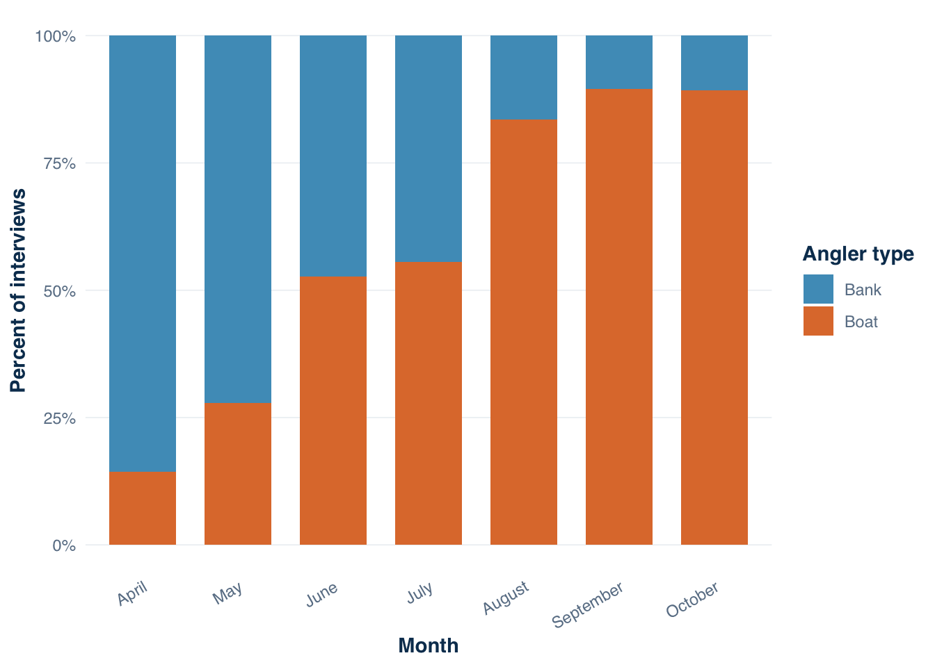
The interview count and percentage by angler type across months appears below. Figure 16.1 then shows the same information as a stacked proportion chart.
       month angler_type   N percent
1      April        bank  18    85.7
2      April        boat   3    14.3
3        May        bank 143    72.2
4        May        boat  55    27.8
5       June        bank  53    47.3
6       June        boat  59    52.7
7       July        bank  40    44.4
8       July        boat  50    55.6
9     August        bank  14    16.5
10    August        boat  71    83.5
11 September        bank   6    10.5
12 September        boat  51    89.5
13   October        bank   4    10.8
14   October        boat  33    89.2
Figure 16.1: Monthly interview composition by angler type at Harlan Reservoir, 2022. Bank angler dominance shifts to boat angler dominance as the season progresses into summer and early fall. Domains that depend on angler type — such as bank vs. boat CPUE — require this variable to be collected on every interview.
Fishing method composition
The method summary follows the same structure, grouping interview counts and percentages by month and fishing method.
Code
summarize_by_method(harlan_design)
Table 16.3
       month        method   N percent
1      April Bow and Arrow   0     0.0
2      April  Rod and Reel  21   100.0
3        May Bow and Arrow   1     0.5
4        May  Rod and Reel 197    99.5
5       June Bow and Arrow   0     0.0
6       June  Rod and Reel 112   100.0
7       July Bow and Arrow   0     0.0
8       July  Rod and Reel  90   100.0
9     August Bow and Arrow   0     0.0
10    August  Rod and Reel  85   100.0
11 September Bow and Arrow   0     0.0
12 September  Rod and Reel  57   100.0
13   October Bow and Arrow   0     0.0
14   October  Rod and Reel  37   100.0
The Harlan survey is nearly all rod-and-reel throughout the season. One bow-fishing interview in May is the only exception. In a mixed-gear fishery — such as a reservoir where night bow fishing is common for rough fish — the angler_method field would enable gear-specific catch rate estimates for each species. The Harlan data illustrate that even when a classification variable shows little variation, recording it is zero-cost insurance: if the fishery changes, the data structure is already in place.
16.5 Schedule compliance
Before moving from the field phase to the analysis phase, confirm that the sampling schedule was executed as planned. validate_creel_schedule() validates the schedule’s required columns and value types, then returns the schedule for inspection. The sampled column records which days were actually sampled.
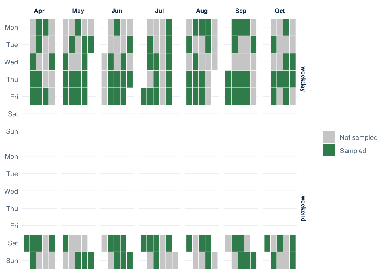
Each row is one day in the season frame. The sampled column is TRUE when at least one interview or count record exists for that date. Figure 16.2 maps the result across the calendar to make gaps visible by month and day type.
Figure 16.2: Harlan Reservoir 2022 sampling schedule coverage by month and day type. Green tiles are sampled days; grey tiles are unsampled days in the season frame. Coverage is consistent within both strata across the season — no systematic gaps in weekend or weekday sampling — confirming that the stratified design executed as planned (see Section 12.12).
Of the 211 days in the Harlan season frame, 116 were sampled and 95 were not. Unsampled days are expected — the design intentionally allocates a subset of available days to avoid field fatigue and budget overrun. What matters is that the unsampled days are random within strata, not systematically tied to weather or fish activity.
If a sampled day appears in the schedule but has zero interviews or counts, validate_creel_schedule() will flag it as not sampled. That situation warrants investigation: was the crew unable to reach the site, or is data missing for another reason?
16.6 Documenting nonresponse
Not every contacted angler agrees to be interviewed. Refusal rates in creel surveys are typically low — under 5% in most freshwater programs — but even low rates can introduce bias if refusers systematically differ from participants (Pollock et al. 1994). Anglers who refuse often do so because they are leaving quickly after a poor trip, which could bias catch rate estimates upward.
The refused column in the interviews table captures whether a contacted party declined the interview. Recording it requires one additional question — “Are you willing to answer a few questions?” — before the standard interview begins.
The example_interviews dataset includes a refused column. Building a design with that column named exposes it to summarize_refusals():
Warning: ! No `n_anglers` provided — assuming 1 angler per interview.
ℹ Pass `n_anglers = <column>` to use actual party sizes for angler-hour
  normalization.
ℹ If the interviews really are one angler each, pass `n_anglers = 1` to state
  that and silence this warning.
  month participation  N percent
1  June      accepted 22     100
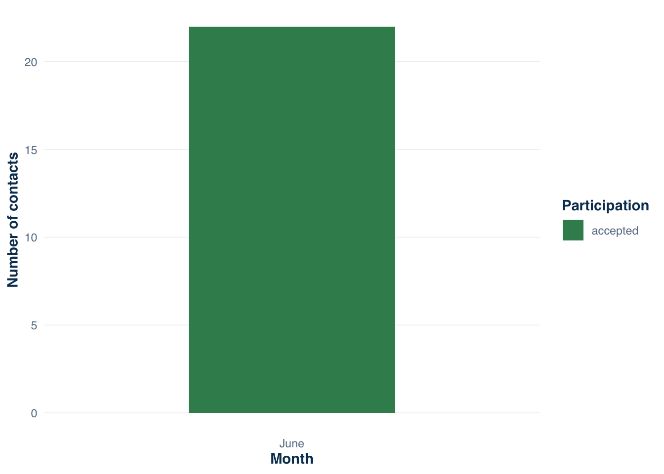
The returned data frame has one row per month per participation category (accepted / refused). All contacts in the example dataset were accepted; Figure 16.3 shows the resulting bar chart and illustrates what a survey with actual refusals would produce.
Code
summarize_refusals(refusal_design) |>mutate(month =factor(month, levels = month.name)) |>ggplot(aes(x = month, y = N, fill = participation)) +geom_col(position ="stack", width =0.5) +scale_fill_manual(values =c("accepted"="#3A8B5B", "refused"="#C0392B"),name ="Participation" ) +labs(x ="Month",y ="Number of contacts" ) +theme_creel()
Figure 16.3: Monthly interview participation rates from the example creel dataset. All contacted anglers agreed to participate in this example survey. In a typical creel program, refused contacts appear alongside accepted contacts, enabling monthly tracking of nonresponse rates.
The Harlan 2022 form did not record refusals, so this analysis uses example_interviews, which includes a refused column. If you plan to assess nonresponse bias — or to apply the adjust_nonresponse() correction from Section 15.4 — the refused flag must be on every form from day one of the survey season.
16.7 Standardization across crews
The same interview form used by different technicians can produce incompatible data if terminology is not standardized. Three fields are especially vulnerable:
Species names. Technicians who record species verbally rather than using standard codes produce strings like "Walleye", "walleye", "Wall Eye", and "Yellow Pike" for the same species. standardize_species() (Section 20.2) resolves these to AFS species codes automatically for most species, but the cleaning burden is proportional to the inconsistency introduced in the field. A laminated species reference card with standard codes — taped to the interview board — eliminates most of this variation at the source.
Trip status values."complete", "Complete", "COMPLETE", "C", and "done" are all plausible entries for a completed trip in a text field. tidycreel expects "complete" and "incomplete". Pre-defined dropdowns or checkboxes on digital forms prevent this; a fixed vocabulary in technician training prevents it on paper.
Angler type. A consistent vocabulary ("bank", "boat") is needed across all technicians, all sites, and all survey years for multi-year domain comparisons to be valid. If one technician codes waders as "bank" and another codes them as "boat", the domain estimate conflates two access types.
Standardization is a data management problem that the form structure can prevent. The schema established in creel_schema() defines the expected values; validation checks after data entry catch violations before analysis begins.
16.8 How form decisions constrain estimation
Table 16.4 summarizes the direct mapping between form design decisions and downstream estimation capability. Each row describes a field that, if omitted, removes a specific estimator or domain from the analysis.
Table 16.4: Field instrument design decisions and their downstream estimation consequences. A missing field cannot be recovered through alternative analysis — the data do not exist. Decisions made before the first sampling day determine what is permanently possible.
If you omit…
You cannot compute…
Workaround?
harvest column (catch_type = ‘harvested’)
Harvest totals, harvest rate, exploitation rate
None — total catch only
trip_status
MOR/ROM estimator selection for CPUE
Assume all complete (access-point surveys only)
hours_fished
CPUE (catch per angler-hour)
None
angler_type
Bank vs. boat domain estimates
None
angler_method
Gear-specific catch rates
None
species_sought
Target-species interview filtering
None
refused flag
Nonresponse rate, nonresponse adjustment
External refusal logs (if kept)
n_anglers (party size)
Party-expansion for total-angler effort
Assume party size = 1
The constraint table is not a checklist of nice-to-have variables. It is a mapping between management questions and instrument requirements. If a regulation revision requires estimating the proportion of catch that is harvested vs. released — a post-season request that could not have been anticipated — and the form recorded only total catch, the analysis is impossible regardless of sample size.
The variables that are hardest to add retroactively — refused, species_sought, harvest as a separate column — are also the ones most likely to be deprioritized in form design discussions because their value is not apparent until after data collection ends. Reviewing Table 16.4 before finalizing the field form, and mapping each “You cannot compute” cell to a real management use case, makes the cost of omission concrete before it is irreversible. Section 15.4 and Section 15.5 cover the bias implications of several of these omissions in more detail.
16.9 Takeaway
The interview and count forms are the first link in the estimation chain. In tidy survey analysis, every downstream function call — estimate_total_harvest(), estimate_catch_rate(by = "angler_type"), adjust_nonresponse() — depends on variables that either exist in the raw data or do not. There is no imputation for a field that was never recorded (Pollock et al. 1994).
Reviewing creel_schema() before a survey season begins, and mapping every schema slot to a specific form question, reduces the risk of discovering a missing variable only after data collection ends. Section 18.1 shows how the resulting raw tables should be structured, and Section 19.1 shows how creel_design() binds them into an analysis-ready object. Before either of those steps, the data must come from somewhere — the subject of the next chapter.
Pollock, K. H., C. M. Jones, and T. L. Brown. 1994. Angler survey methods and their applications in fisheries management. American Fisheries Society, Bethesda, Maryland.