13  Pre-Survey Planning: Sample Size and Schedule Design

Keywords

creel survey, fisheries, design-based inference, R, tidycreel, Quarto

A creel survey that finishes the season with a 45% CV on the effort estimate has not merely underperformed — it has wasted field resources and produced information that cannot support management decisions. The time to prevent that outcome is before the first count sheet is printed, not after the data have been collected. Pre-survey planning translates management objectives into concrete resource commitments: how many sampling days, how many angler interviews, and when to schedule them.

This chapter covers the prospective side of survey design. Where Chapter 15 asks “how precise was my estimate?”, this chapter asks “how many sampling units do I need to achieve a target precision?” The two questions are mirrors of each other, and tidycreel provides a dedicated suite of functions for both.

13.1 The planning inputs

Three quantities are needed before any sample size calculation can be run.

A precision target. Agency standards differ, but a coefficient of variation (CV) of 20% or less is widely cited as the threshold for a management-grade creel estimate (Pollock et al. 1994; McCormick and Meyer 2017). A target CV of 15% is more demanding but achievable on productive fisheries with moderate sampling effort. The CV target must be stated before the survey begins; setting it retrospectively invites motivated reasoning.

A stratification frame (N_h). The total number of eligible sampling days per stratum — the frame — bounds how much precision is achievable regardless of effort. For a day-type-stratified survey, N_h comes from the season calendar: count the weekdays and weekend days in the planned season window.

Pilot variance estimates (ybar_h, s2_h). Sample size formulas require between-day variance within each stratum. For a new fishery with no prior data, the literature suggests starting with a budget of approximately 30 sampling days and iterating (McCormick and Meyer 2017). For an established program, historical data from previous seasons provide reliable variance estimates.

The Harlan reservoir survey has been running long enough that a completed season can serve as the pilot for planning the next one. The following chunk extracts the three planning inputs from the 2022 Harlan data.

# Shift lengths: period 1 = AM (8 h), period 2 = PM (6 h)
shift_hours <- c("1" = 8L, "2" = 6L)

daily_effort <- harlan_counts |>
  mutate(
    period       = as.character(period),
    angler_hours = (boat_anglers + bank_anglers) * shift_hours[period]
  ) |>
  group_by(date, day_type) |>
  summarise(daily_effort = sum(angler_hours), .groups = "drop")

pilot_stats <- daily_effort |>
  group_by(day_type) |>
  summarise(
    n_sampled = n(),
    ybar      = mean(daily_effort),    # mean effort per sampled day
    s2        = var(daily_effort),     # between-day variance
    .groups   = "drop"
  )

pilot_stats

# A tibble: 2 × 4
  day_type n_sampled  ybar      s2
  <chr>        <int> <dbl>   <dbl>
1 weekday         83  375. 161734.
2 weekend         35  162.  54123.

# Season frame: eligible days per stratum
N_h <- harlan_schedule |>
  group_by(day_type) |>
  summarise(N = n(), .groups = "drop")

N_h

# A tibble: 2 × 2
  day_type     N
  <chr>    <int>
1 weekday    150
2 weekend     61

The Harlan 2022 season ran across 211 calendar days: 150 weekdays and 61 weekend/holiday days. Weekday effort is on average more than twice the weekend mean (375 vs 162 angler-hours per sampled day), and between-day variance is correspondingly larger in the weekday stratum.

These six values — N_h, ybar_h, and s2_h for each of the two strata — are everything creel_n_effort() needs.

13.2 How many sampling days?

creel_n_effort() implements the stratified sample size formula from McCormick and Meyer (2017), based on Cochran ((1977)) eq. 5.25. It returns the total number of sampling days needed to achieve a target CV on the effort estimate, along with the proportional allocation of those days to each stratum.

N_hv    <- setNames(N_h$N,          N_h$day_type)
ybar_hv <- setNames(pilot_stats$ybar, pilot_stats$day_type)
s2_hv   <- setNames(pilot_stats$s2,  pilot_stats$day_type)

creel_n_effort(cv_target = 0.20, N_h = N_hv, ybar_h = ybar_hv, s2_h = s2_hv)

weekday weekend   total 
     20       9      28 

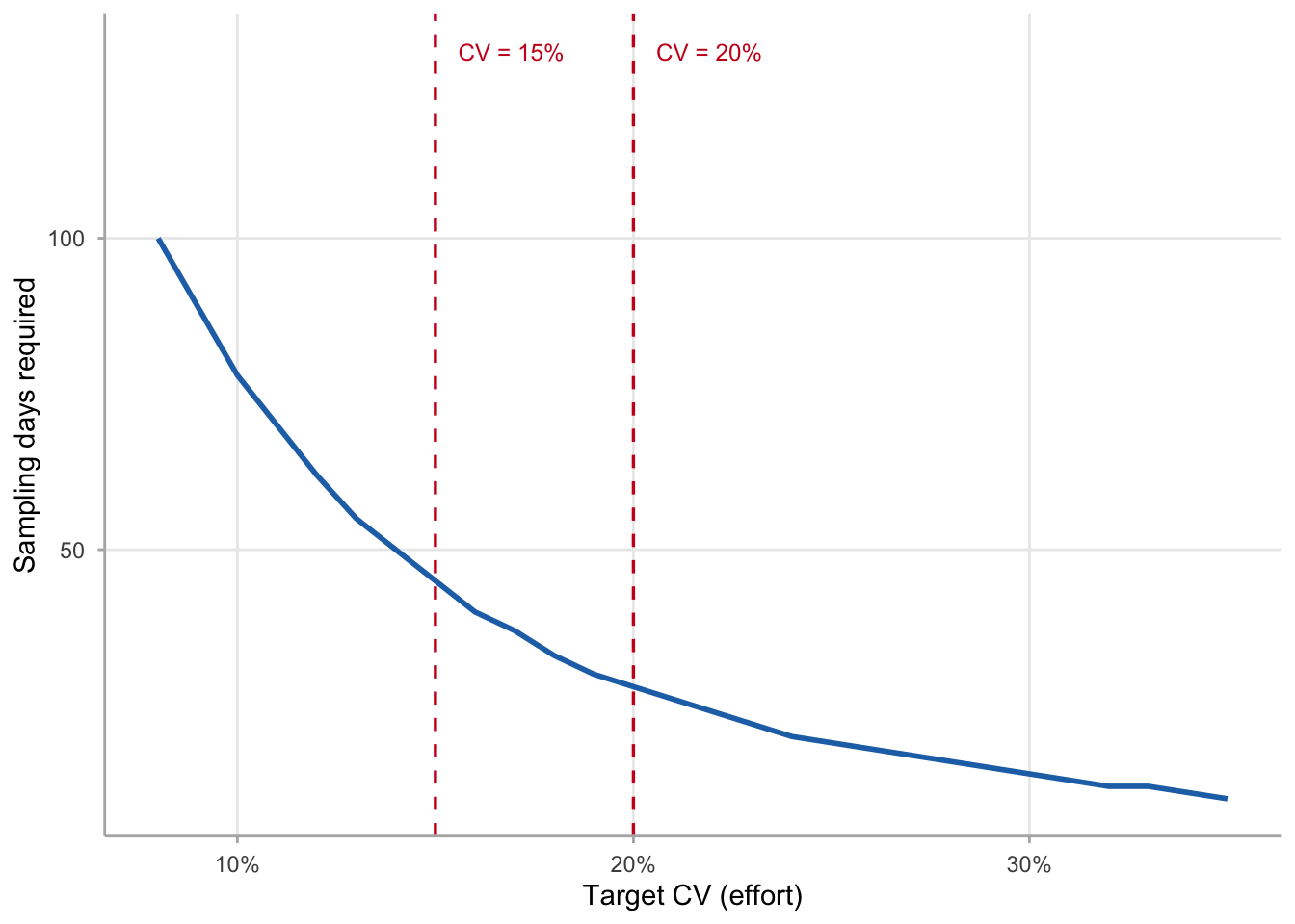
Twenty-eight sampling days are sufficient to hit a 20% CV on effort for the Harlan 2022 design. Of those, 20 fall in the weekday stratum and 9 in the weekend stratum, reflecting proportional allocation to season length. Tightening the target to 15% requires 45 days:

# Range of CV targets
cv_targets <- c(0.10, 0.15, 0.20, 0.25)

purrr::map(
  cv_targets,
  ~ creel_n_effort(.x, N_hv, ybar_hv, s2_hv)
) |>
  purrr::set_names(paste0("CV = ", cv_targets)) |>
  purrr::map_dfr(~ as.list(.x), .id = "cv_target") |>
  select(cv_target, weekday, weekend, total)

# A tibble: 4 × 4
  cv_target weekday weekend total
  <chr>       <int>   <int> <int>
1 CV = 0.1       56      23    78
2 CV = 0.15      32      14    45
3 CV = 0.2       20       9    28
4 CV = 0.25      14       6    19

The relationship between CV target and required days follows a familiar pattern: precision improves rapidly at first, then diminishing returns set in. Cutting the CV from 25% to 20% costs only 9 additional sampling days; cutting it from 15% to 10% costs 33 more. This trade-off is most clearly seen as a curve.

tradeoff <- tibble(cv_target = seq(0.08, 0.35, by = 0.01)) |>
  mutate(
    result  = purrr::map(cv_target, ~ creel_n_effort(.x, N_hv, ybar_hv, s2_hv)),
    n_total = purrr::map_int(result, ~ .x["total"])
  )

thresholds <- tibble(
  cv_target = c(0.15, 0.20),
  label     = c("CV = 15%", "CV = 20%")
)

ggplot(tradeoff, aes(x = cv_target * 100, y = n_total)) +
  geom_line(colour = "#2171b5", linewidth = 1) +
  geom_vline(
    data    = thresholds,
    aes(xintercept = cv_target * 100),
    linetype = "dashed",
    colour   = "#cb181d",
    linewidth = 0.6
  ) +
  geom_label(
    data  = thresholds,
    aes(x = cv_target * 100 + 0.4, y = 130, label = label),
    colour = "#cb181d",
    size   = 3.2,
    hjust  = 0,
    label.size = 0
  ) +
  scale_x_continuous(labels = function(x) paste0(x, "%")) +
  labs(
    x = "Target CV (effort)",
    y = "Sampling days required"
  ) +
  theme_creel()

Warning: The `label.size` argument of `geom_label()` is deprecated as of ggplot2 3.5.0.
ℹ Please use the `linewidth` argument instead.

Figure 13.1: Required sampling days versus target effort CV. Diminishing returns are steep: each incremental gain in precision demands disproportionately more sampling days. Reference lines mark commonly used agency thresholds.

An important caveat: these sample sizes are minimums under the assumption that observations are distributed according to the pilot variances. Real variances fluctuate between years. A prudent practice is to add a 10–15% buffer to the computed minimum or to re-run the calculation mid-season if conditions differ substantially from the pilot year.

13.3 How many interviews?

Effort precision is driven by the number of sampling days. CPUE precision is driven by the number of angler interviews. The two sample sizes are independent because they estimate different things: effort uses count data collected by surveyors, while CPUE uses per-party catch and effort reported by anglers.

creel_n_cpue() computes the number of interviews required to achieve a target CV on the CPUE ratio estimator (Cochran 1977, Ch. 6). It requires pilot CVs for catch and effort per interview, plus the correlation between them.

catch_by_interview <- harlan_catch |>
  group_by(interview_id) |>
  summarise(n_fish = sum(n_fish), .groups = "drop")

interviews_pilot <- harlan_interviews |>
  left_join(catch_by_interview, by = "interview_id") |>
  mutate(n_fish = if_else(is.na(n_fish), 0L, as.integer(n_fish)))

cv_catch  <- sd(interviews_pilot$n_fish)    / mean(interviews_pilot$n_fish)
cv_effort <- sd(interviews_pilot$hours_fished) / mean(interviews_pilot$hours_fished)
rho       <- cor(interviews_pilot$n_fish, interviews_pilot$hours_fished)

tibble(
  statistic = c("CV of catch per interview", "CV of effort per interview", "Correlation (rho)"),
  value     = round(c(cv_catch, cv_effort, rho), 3)
)

# A tibble: 3 × 2
  statistic                  value
  <chr>                      <dbl>
1 CV of catch per interview  1.62 
2 CV of effort per interview 0.738
3 Correlation (rho)          0.347

Catch is highly variable relative to its mean (CV ≈ 1.6), which is typical of recreational fisheries: most parties catch nothing while a few catch many fish. Effort (hours fished per party) is less dispersed (CV ≈ 0.7). The positive correlation between catch and effort (ρ ≈ 0.35) means that parties who fish longer also tend to catch more — a signal of behavioral variation across angler types.

# Conservative estimate (rho = 0 over-estimates n when catch and effort covary)
creel_n_cpue(
  cv_catch  = cv_catch,
  cv_effort = cv_effort,
  rho       = 0,
  cv_target = 0.20
)

[1] 80

# Less conservative: use observed correlation
creel_n_cpue(
  cv_catch  = cv_catch,
  cv_effort = cv_effort,
  rho       = rho,
  cv_target = 0.20
)

[1] 59

Setting rho = 0 is conservative: it over-estimates the required sample size because it ignores the variance-reducing effect of positive catch–effort covariance. The observed ρ = 0.35 reduces the 20%-CV interview requirement from 80 to 59. Using the observed correlation is appropriate when pilot data are reliable; in the absence of pilot data, the conservative rho = 0 default is the safer choice.

A practical minimum of 100 interviews is also widely recommended. Below that threshold, the ratio estimator’s confidence interval coverage may fall short of its nominal 95% even if the formula suggests fewer interviews are needed, because the distribution of catch per angler is highly right-skewed (Pollock et al. 1994).

13.4 Working backwards from a fixed budget

Planning calculations usually run in the forward direction: “I need CV = 20%; how many days?” But managers sometimes allocate a fixed number of sampling days before the precision question is asked, and the analyst must then characterize what that budget can deliver.

cv_from_n() inverts the sample size formula: given a fixed number of sampling units, what CV should you expect? Set type = "cpue" for interviews or type = "effort" for sampling days.

# Director approves 60 interviews: what CPUE CV is achievable?
cv_from_n(
  type      = "cpue",
  n         = 60L,
  cv_catch  = cv_catch,
  cv_effort = cv_effort,
  rho       = 0   # conservative
)

[1] 0.2296915

cv_from_n(
  type      = "cpue",
  n         = 100L,
  cv_catch  = cv_catch,
  cv_effort = cv_effort,
  rho       = 0
)

[1] 0.1779183

Sixty interviews delivers an expected CPUE CV of about 23%, which may exceed the agency’s 20% threshold. One hundred interviews brings the CV to 18%, comfortably within standard precision targets. If neither budget is achievable, this output makes the trade-off explicit and auditable — a more defensible position than an after-the-fact rationalization of inadequate precision.

13.5 Allocating days across strata

Once the total number of sampling days is determined, they must be distributed across strata. Two allocation strategies dominate creel survey practice: proportional allocation assigns days in proportion to each stratum’s share of the season calendar; Neyman (optimal) allocation directs more days to strata with higher between-day variance, minimizing total variance for a fixed sample budget (Cochran 1977; Pollock et al. 1994).

reallocate_strata() computes Neyman-optimal allocation given a fixed day budget and stratum-level pilot variances.

n_budget <- 45L   # total sampling days available

# Proportional allocation
prop_alloc <- round(n_budget * N_hv / sum(N_hv)) |>
  as.integer() |>
  setNames(names(N_hv))

# Neyman-optimal allocation
neyman_alloc <- reallocate_strata(n_total = n_budget, N_h = N_hv, s2_h = s2_hv)

tibble(
  stratum  = names(N_hv),
  N_h      = as.integer(N_hv),
  prop     = prop_alloc,
  neyman   = neyman_alloc[names(N_hv)]
)

# A tibble: 2 × 4
  stratum   N_h  prop neyman
  <chr>   <int> <int>  <int>
1 weekday   150    32     37
2 weekend    61    13      9

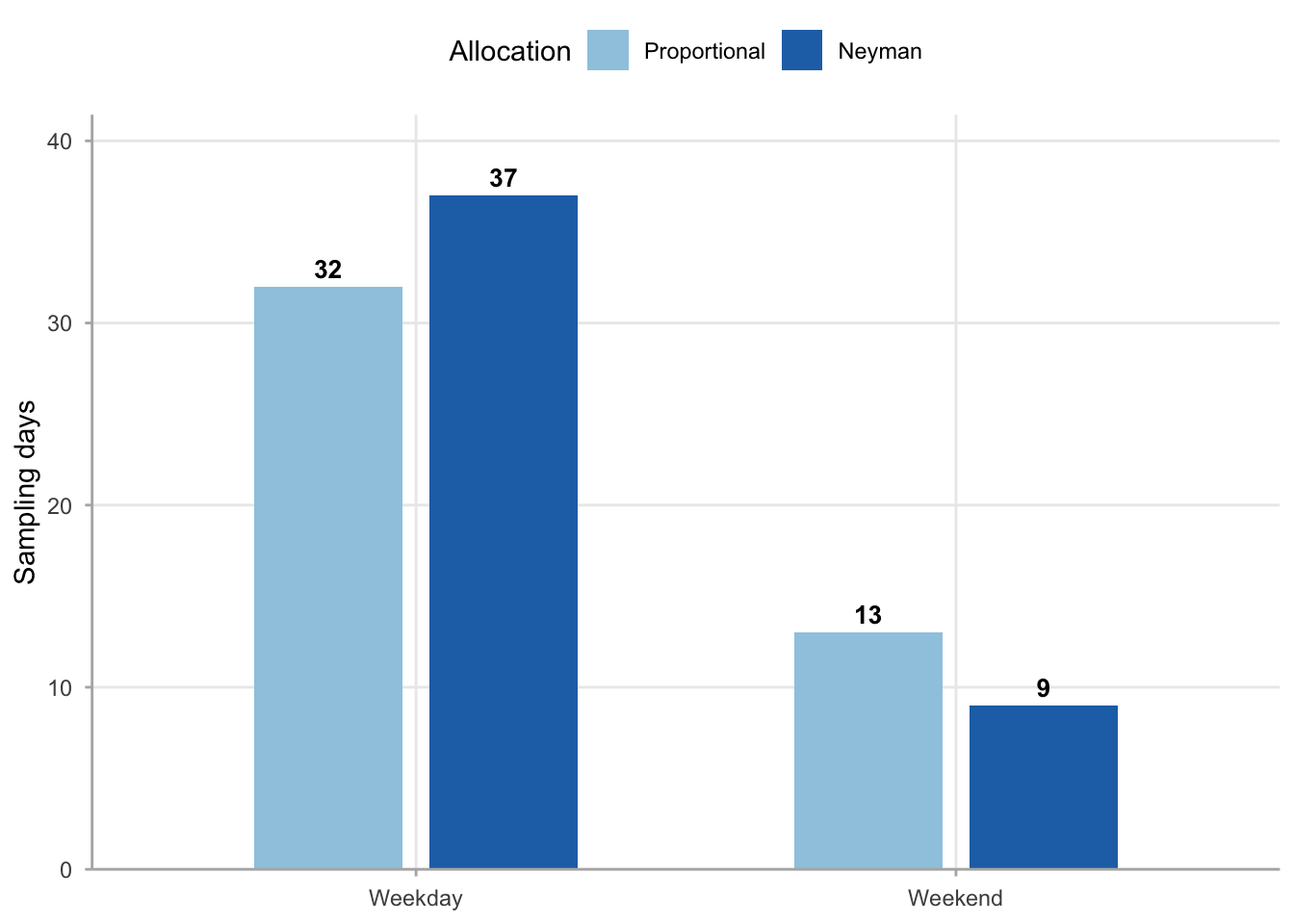
For the Harlan design, Neyman allocation adds 5 days to the weekday stratum and removes 4 from the weekend stratum relative to proportional (32→37 weekday, 13→9 weekend). The weekday stratum has both more calendar days and substantially higher between-day variance (161,734 vs 54,123), so directing additional sampling effort there reduces the overall variance of the effort estimate.

alloc_df <- tibble(
  stratum    = rep(c("Weekday", "Weekend"), 2),
  method     = rep(c("Proportional", "Neyman"), each = 2),
  n_days     = c(prop_alloc["weekday"], prop_alloc["weekend"],
                 neyman_alloc["weekday"], neyman_alloc["weekend"])
) |>
  mutate(method = factor(method, levels = c("Proportional", "Neyman")))

ggplot(alloc_df, aes(x = stratum, y = n_days, fill = method)) +
  geom_col(position = position_dodge(width = 0.65), width = 0.55) +
  geom_text(
    aes(label = n_days),
    position = position_dodge(width = 0.65),
    vjust    = -0.5,
    size     = 3.5,
    fontface = "bold"
  ) +
  scale_fill_manual(values = c("Proportional" = "#9ecae1", "Neyman" = "#2171b5")) +
  scale_y_continuous(expand = expansion(mult = c(0, 0.12))) +
  labs(x = NULL, y = "Sampling days", fill = "Allocation") +
  theme_creel() +
  theme(legend.position = "top")

Figure 13.2: Proportional versus Neyman allocation of 45 sampling days across day-type strata. Neyman allocation concentrates effort in the weekday stratum, which has both more eligible days and higher between-day variance.

Neyman allocation is most beneficial when strata differ substantially in variance. When strata have similar within-stratum variability, proportional allocation performs nearly as well and has the practical advantage of simplicity: interviewers can be scheduled without knowledge of historical variance estimates, and the allocation is easier to explain to field crews and managers.

optimal_n() combines the two steps — total sample size and Neyman allocation — into a single call. Rather than first computing creel_n_effort() and then calling reallocate_strata(), optimal_n() takes the CV target directly and returns both the required total days and the per-stratum allocation:

optimal_alloc <- optimal_n(
  cv_target = 0.20,
  N_h       = N_hv,
  ybar_h    = ybar_hv,
  s2_h      = s2_hv
)
optimal_alloc

weekday weekend   total 
     23       6      28 

The result shows total days required under Neyman allocation to hit the target CV, alongside the per-stratum breakdown. For the Harlan design, optimal_n() returns the same total (28) as creel_n_effort() at this CV target, but allocates differently: 23 weekday / 6 weekend (Neyman) versus 20 weekday / 9 weekend (proportional). Neyman allocation concentrates days in the weekday stratum because that stratum has both more calendar days and higher between-day variance. When strata variances differ substantially across surveys, Neyman allocation can require fewer total days than proportional for the same precision target; for the Harlan design the totals happen to be equal, and the practical benefit is the more efficient per-stratum split.

13.6 Power to detect a change

CV targets address precision, not the capacity to detect change. A survey that delivers a 20% CV on a seasonal CPUE estimate can still fail to detect a biologically important regulation effect if individual catch rates are highly variable. creel_power() calculates the probability of detecting a fractional change in CPUE between two seasons given the number of interviews per season, the historical CV of individual CPUE measurements, and a significance threshold.

The key input is cv_historical: the coefficient of variation of CPUE measured from individual interviews (fish per hour per completed trip). This reflects how heterogeneous anglers are — a fishery where most parties catch similar amounts has a low CV; one where a few parties catch most of the fish has a high CV. For Harlan:

# CV of CPUE per completed interview (fish per hour)
cpue_per_interview <- harlan_interviews |>
  left_join(
    harlan_catch |>
      group_by(interview_id) |>
      summarise(n_fish = sum(n_fish), .groups = "drop"),
    by = "interview_id"
  ) |>
  mutate(n_fish = if_else(is.na(n_fish), 0L, as.integer(n_fish))) |>
  filter(trip_status == "complete", hours_fished > 0) |>
  mutate(cpue = n_fish / hours_fished)

cv_historical <- sd(cpue_per_interview$cpue) / mean(cpue_per_interview$cpue)
round(cv_historical, 2)

[1] 2.66

Harlan’s CV of 2.66 is typical of multi-species recreational fisheries where zero-catch parties are common: the distribution of individual catch rates is strongly right-skewed, driving up the standard deviation relative to the mean. High cv_historical means that detecting a moderate regulation effect requires substantially more interviews than the precision target alone implies.

# 390 interviews is the approximate Harlan annual sample
creel_power(
  n             = 390L,
  cv_historical = cv_historical,
  delta_pct     = 0.20,
  alpha         = 0.05,
  alternative   = "two.sided"
)

[1] 0.182395

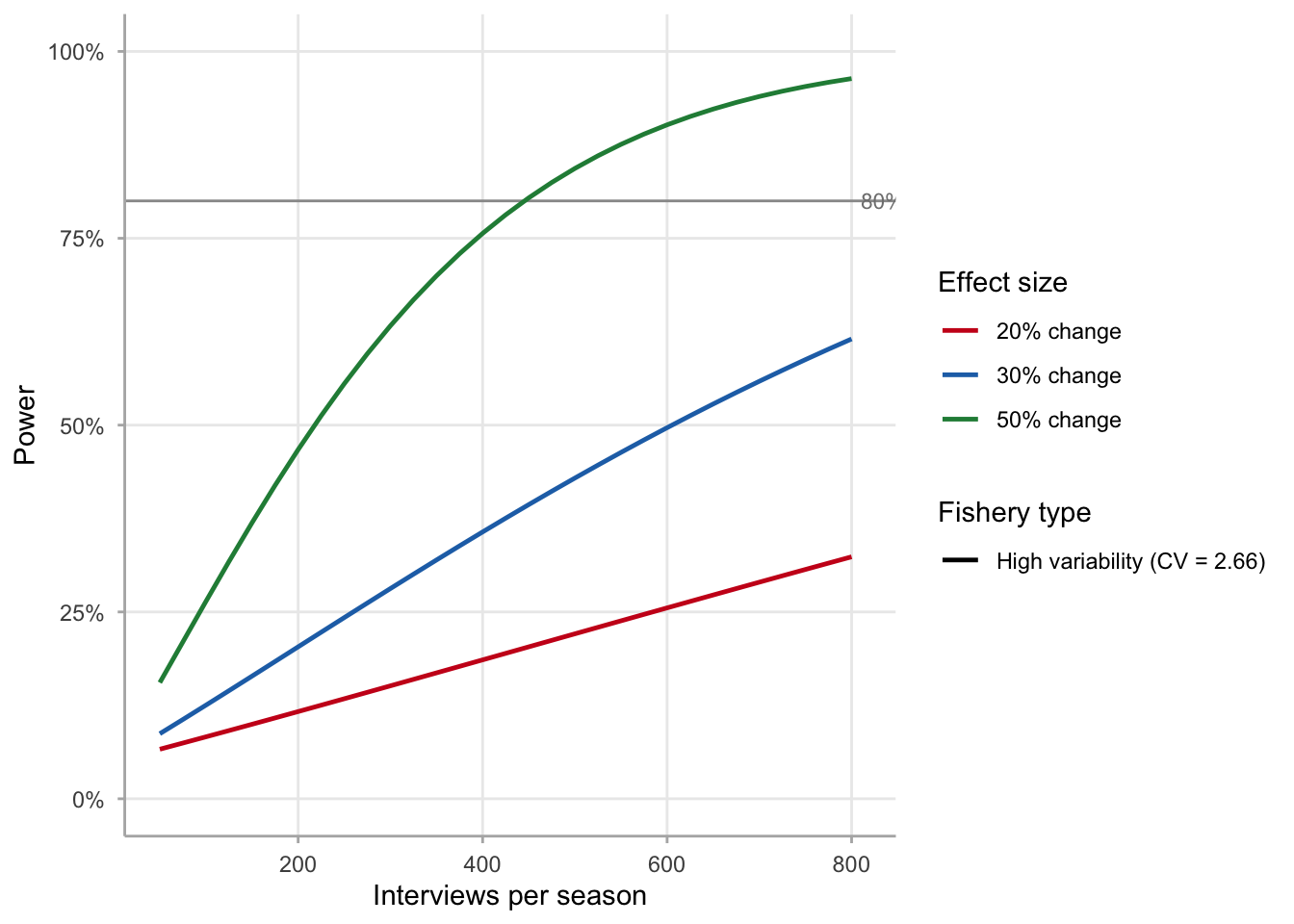
With 390 interviews per season — the approximate Harlan annual sample — power to detect a 20% CPUE change is only about 18%. Even a 50% change is below 80% power at that sample size:

creel_power(
  n             = 390L,
  cv_historical = cv_historical,
  delta_pct     = 0.50,
  alpha         = 0.05,
  alternative   = "two.sided"
)

[1] 0.7459632

This is not a failure of the Harlan survey design; it reflects the inherent difficulty of detecting moderate changes in CPUE when individual catch rates are heterogeneous. The power curve illustrates how detection threshold depends on both sample size and individual-level variability.

power_grid <- expand.grid(
  n             = seq(50, 800, by = 25),
  delta_pct     = c(0.20, 0.30, 0.50),
  cv_hist       = c(cv_historical, 0.80)
) |>
  as_tibble() |>
  mutate(
    power = purrr::pmap_dbl(
      list(n, delta_pct, cv_hist),
      function(n_i, d_i, cv_i)
        creel_power(n_i, cv_historical = cv_i, delta_pct = d_i, alpha = 0.05)
    ),
    delta_label = paste0(delta_pct * 100, "% change"),
    fishery     = if_else(
      cv_hist > 1,
      paste0("High variability (CV = ", round(cv_hist, 2), ")"),
      paste0("Low variability (CV = ", round(cv_hist, 2), ")")
    )
  )

ltype_vals <- c("solid", "dashed") |>
  setNames(c(
    paste0("High variability (CV = ", round(cv_historical, 2), ")"),
    "Low variability (CV = 0.80)"
  ))

ggplot(power_grid, aes(
  x        = n,
  y        = power,
  colour   = delta_label,
  linetype = fishery
)) +
  geom_hline(yintercept = 0.80, colour = "grey60", linewidth = 0.5) +
  annotate("text", x = 810, y = 0.80, label = "80%", hjust = 0, size = 3, colour = "grey50") +
  geom_line(linewidth = 0.85) +
  scale_colour_manual(
    values = c("20% change" = "#cb181d", "30% change" = "#2171b5", "50% change" = "#238b45"),
    name   = "Effect size"
  ) +
  scale_linetype_manual(values = ltype_vals, name = "Fishery type") +
  scale_y_continuous(labels = scales::percent_format(accuracy = 1), limits = c(0, 1)) +
  scale_x_continuous(breaks = seq(0, 800, by = 200)) +
  labs(x = "Interviews per season", y = "Power") +
  theme_creel() +
  theme(legend.position = "right")

Warning: Removed 93 rows containing missing values or values outside the scale range
(`geom_line()`).

Figure 13.3: Statistical power to detect a fractional CPUE change as a function of interviews per season, for three effect sizes. Solid curves use the Harlan pilot CV (2.66); dashed curves show a hypothetical lower-variance fishery (CV = 0.80) as a contrast. Power is calculated using a two-sided normal approximation at α = 0.05.

Two contrasts stand out. First, for the low-variance fishery (CV = 0.80, dashed), 80% power to detect a 30% change requires only about 120 interviews — a feasible season target. For Harlan (CV = 2.66, solid), the same target requires more than 1,200 interviews per season. Second, a 50% CPUE change is detectable with 80% power at approximately 450 interviews for Harlan — a large but not impossible sample if the survey priority justifies it.

The practical implication: power analysis for CPUE change detection should be conducted early in the planning cycle, before interview targets are set, so that resource decisions reflect the actual detection capacity of the survey. A survey with adequate precision (CV ≤ 20%) may still have limited power to detect realistic regulation effects on heterogeneous fisheries.

13.7 Translating days to a calendar

Sample size outputs are unitless numbers: “sample 32 weekdays and 14 weekend days.” Turning those numbers into a field schedule requires randomly assigning specific dates within each stratum across the season window. generate_schedule() does this: it takes a date range and stratum-specific day counts and returns a stratified random sample of survey dates.

planned_schedule <- generate_schedule(
  start_date = "2023-04-01",
  end_date   = "2023-10-31",
  n_periods  = 2,
  n_days     = c(weekday = 32L, weekend = 14L),
  include_all = FALSE,
  seed        = 2024
)

planned_schedule

April 2023

Sun	Mon	Tue	Wed	Thu	Fri	Sat
						01
WEEKE	03	04	WEEKD	06	07	08
09	WEEKD	11	12	13	14	15
16	17	18	19	20	21	22
23	24	25	26	27	WEEKD	29
30

May 2023

Sun	Mon	Tue	Wed	Thu	Fri	Sat
	01	02	03	04	WEEKD	WEEKE
07	WEEKD	09	WEEKD	11	12	13
WEEKE	15	WEEKD	17	WEEKD	WEEKD	20
WEEKE	22	23	24	25	26	WEEKE
28	29	30	31

June 2023

Sun	Mon	Tue	Wed	Thu	Fri	Sat
				01	02	03
04	05	06	WEEKD	WEEKD	WEEKD	10
11	12	13	14	WEEKD	16	17
18	19	WEEKD	21	22	23	24
25	26	27	28	29	WEEKD

July 2023

Sun	Mon	Tue	Wed	Thu	Fri	Sat
						01
02	03	WEEKD	05	06	07	WEEKE
09	10	11	12	13	14	15
WEEKE	17	18	19	20	WEEKD	22
WEEKE	WEEKD	25	26	WEEKD	28	29
30	31

August 2023

Sun	Mon	Tue	Wed	Thu	Fri	Sat
		WEEKD	02	03	WEEKD	WEEKE
06	07	08	09	10	11	12
13	14	15	16	17	18	WEEKE
20	21	22	23	24	WEEKD	26
27	WEEKD	29	30	31

September 2023

Sun	Mon	Tue	Wed	Thu	Fri	Sat
					01	WEEKE
03	04	05	06	07	08	09
10	WEEKD	12	13	14	15	16
17	18	19	20	WEEKD	22	23
24	25	26	27	WEEKD	29	30

October 2023

Sun	Mon	Tue	Wed	Thu	Fri	Sat
WEEKE	02	WEEKD	04	05	WEEKD	WEEKE
08	WEEKD	10	11	12	WEEKD	14
15	16	17	WEEKD	19	20	21
WEEKE	23	24	25	WEEKD	27	28
29	30	31

The output is a creel_schedule object with one row per sampled day × period — ready to pass directly to creel_design() when the survey begins. A quick diagnostic check confirms that the selected days spread reasonably across the season.

planned_schedule |>
  mutate(month = lubridate::month(date, label = TRUE, abbr = TRUE)) |>
  distinct(date, day_type, month) |>
  count(month, day_type) |>
  mutate(day_type = case_match(day_type, "weekday" ~ "Weekday", "weekend" ~ "Weekend")) |>
  ggplot(aes(x = month, y = n, fill = day_type)) +
  geom_col(position = "stack", width = 0.65) +
  scale_fill_manual(values = c("Weekday" = "#2171b5", "Weekend" = "#9ecae1")) +
  scale_y_continuous(breaks = 0:10) +
  labs(x = NULL, y = "Sampling days", fill = "Day type") +
  theme_creel() +
  theme(legend.position = "top")

Warning: There was 1 warning in `mutate()`.
ℹ In argument: `day_type = case_match(day_type, "weekday" ~ "Weekday",
  "weekend" ~ "Weekend")`.
Caused by warning:
! `case_match()` was deprecated in dplyr 1.2.0.
ℹ Please use `recode_values()` instead.

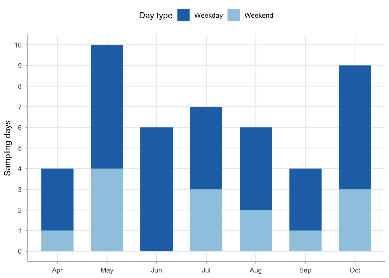
Figure 13.4: Distribution of planned sampling days by month and day type from the generated 2023 Harlan schedule. Stratified random selection spreads days across the April–October season without heavy concentration in any single month.

The stratified random selection ensures that sampled days are spread across the season rather than concentrated in any one month, which protects against confounding seasonal variation with stratum effects.

If the season window shifts or some dates become unavailable (access closures, equipment failure), generate_schedule() can be re-run with a new seed to produce a replacement schedule. Each call produces a statistically valid design as long as the selected dates remain a random sample within strata.

13.8 A planning workflow for the 2023 Harlan season

The six functions form a decision sequence. Below is the complete planning workflow for a hypothetical 2023 Harlan season, using 2022 as the pilot year.

Step 1 — Set precision targets.

targets <- tibble(
  estimand   = c("Effort",       "CPUE"),
  cv_target  = c(0.15,           0.20),
  rationale  = c("management-grade effort estimate", "ratio-estimator precision for CPUE")
)
targets

# A tibble: 2 × 3
  estimand cv_target rationale                         
  <chr>        <dbl> <chr>                             
1 Effort        0.15 management-grade effort estimate  
2 CPUE          0.2  ratio-estimator precision for CPUE

Step 2 — Compute required sampling units.

n_effort <- creel_n_effort(
  cv_target = 0.15,
  N_h       = N_hv,
  ybar_h    = ybar_hv,
  s2_h      = s2_hv
)

n_cpue <- creel_n_cpue(
  cv_catch  = cv_catch,
  cv_effort = cv_effort,
  rho       = 0,
  cv_target = 0.20
)

tibble(
  resource          = c("Sampling days (effort)", "Angler interviews (CPUE)"),
  required          = c(n_effort["total"],         n_cpue),
  practical_minimum = c(30L,                       100L)
)

# A tibble: 2 × 3
  resource                 required practical_minimum
  <chr>                       <int>             <int>
1 Sampling days (effort)         45                30
2 Angler interviews (CPUE)       80               100

Step 3 — Check against budget and revise if needed.

The 45-day effort target and 80-interview CPUE target are both feasible for a season-long Harlan survey. If the field budget supports only 30 sampling days, cv_from_n() characterizes the precision achievable at that budget for both effort and CPUE:

# What effort CV is achievable with 30 sampling days?
cv_from_n(
  type   = "effort",
  n      = 30L,
  N_h    = N_hv,
  ybar_h = ybar_hv,
  s2_h   = s2_hv
)

[1] 0.2106217

Thirty days yields a higher effort CV than the 20% target, making the precision trade-off explicit and auditable before the field season begins. The same call with type = "cpue" and n = 60 or n = 100 was shown earlier in Section 13.4.

Step 4 — Choose an allocation strategy.

final_alloc <- reallocate_strata(
  n_total = n_effort["total"],
  N_h     = N_hv,
  s2_h    = s2_hv
)

tibble(
  stratum = names(final_alloc),
  n_days  = as.integer(final_alloc)
)

# A tibble: 2 × 2
  stratum n_days
  <chr>    <int>
1 weekday     37
2 weekend      9

Step 5 — Generate the field calendar.

field_schedule <- generate_schedule(
  start_date = "2023-04-01",
  end_date   = "2023-10-31",
  n_periods  = 2,
  n_days     = as.integer(final_alloc) |> setNames(names(final_alloc)),
  include_all = FALSE,
  seed        = 99
)

# Summary counts by day_type and month
field_schedule |>
  mutate(month = lubridate::month(date, label = TRUE)) |>
  group_by(day_type, month) |>
  summarise(days_scheduled = n_distinct(date), .groups = "drop") |>
  tidyr::pivot_wider(names_from = day_type, values_from = days_scheduled, values_fill = 0L)

# A tibble: 7 × 3
  month weekday weekend
  <ord>   <int>   <int>
1 Apr         5       0
2 May         4       0
3 Jun         7       1
4 Jul         7       3
5 Aug         6       2
6 Sep         5       2
7 Oct         3       1

The calendar table shows how the 46 allocated sampling days distribute across strata and months (Neyman integer rounding adds one day above the 45-day target). A roughly even spread across the April–October window is desirable; heavy concentration in any one month would bias estimates toward conditions in that month. If a gap appears — for instance, no weekend days scheduled in June — generate_schedule() can be re-run with different seeds until a more balanced calendar is produced, or n_days can be specified per month by using the period_intensity argument.

13.9 What to do without pilot data

Not every new survey has a historical season to draw on. Three options exist in order of preference:

1. Conduct a short pilot study — 10–15 sampling days spread across the season will produce rough variance estimates sufficient for planning purposes. The resulting sample sizes will be uncertain, but the direction of error is known: early-season variance often underestimates full-season variance in temperate fisheries.

2. Borrow from a similar fishery — If a nearby reservoir with comparable species composition and angler density has historical creel data, its within-stratum variance can serve as a proxy. Adjust upward if the target fishery is expected to be more heterogeneous.

3. Use the literature defaults — McCormick and Meyer (2017) report that across 17 inland fisheries, a median of 16 sampling days achieved a 40% relative 95% CI for effort, and approximately 30 days is a reasonable starting point when variance is unknown. For CPUE, a minimum of 100 interviews provides adequate CI coverage even under highly skewed catch distributions (Pollock et al. 1994).

None of these options is as reliable as observed pilot data from the target fishery. But planning under uncertainty is still better than no planning: a 30-day default budget forces an explicit precision conversation before the field season begins, rather than a post-hoc reckoning with an inadequate estimate.

13.10 tidycreel support

Function	Purpose
creel_n_effort()	Sampling days for a target effort CV (proportional allocation)
creel_n_cpue()	Interviews for a target CPUE CV
cv_from_n()	Expected CV given a fixed number of sampling units; type = "effort" or type = "cpue"
optimal_n()	Sampling days and Neyman-optimal per-stratum allocation for a target effort CV
reallocate_strata()	Neyman-optimal allocation across strata given a fixed day budget
creel_power()	Power to detect a fractional CPUE change
generate_schedule()	Stratified random sampling calendar
generate_progressive_start()	Randomised circuit start times for progressive count surveys (discrete or wraparound strategy); avoids the U[0, T − τ] mid-day bias error per Hoenig et al. (1993)

All functions that take stratum-level arguments expect named vectors. Names must match across N_h, ybar_h, and s2_h; mismatched names will produce an error. The output of generate_schedule() is a creel_schedule object that passes directly to creel_design() without further transformation. For roving surveys using progressive counts, generate_progressive_start() produces a companion table of circuit start times and travel directions to be recorded in the field protocol alongside the schedule.

13.11 Takeaway

Pre-survey planning converts management objectives into field commitments. creel_n_effort() answers the effort question; creel_n_cpue() answers the CPUE question; reallocate_strata() distributes days optimally across strata; creel_power() tests whether the planned effort is sufficient to detect biologically important changes; and generate_schedule() turns the numerical targets into a concrete field calendar. For roving surveys that use progressive counts, generate_progressive_start() schedules unbiased circuit start times from the randomised pool defined by the survey period and circuit time.

The Harlan example illustrates a realistic planning sequence: 45 sampling days under Neyman allocation (37 weekday, 9 weekend) will achieve approximately 15% CV on effort, and 80–100 interviews will achieve approximately 20% CV on CPUE. However, the power analysis reveals an important limitation: because individual catch rates are highly variable (CV ≈ 2.66), detecting a moderate CPUE change between seasons requires far more interviews than the precision target implies. Precision and power are related but distinct objectives, and the planning workflow must address both before the first field day is scheduled.

Cochran, W. G. 1977. Sampling techniques, 3rd edition. John Wiley & Sons, New York.

Hoenig, J. M., D. S. Robson, C. M. Jones, and K. H. Pollock. 1993. Scheduling counts in the instantaneous and progressive count methods for estimating sportfishing effort. North American Journal of Fisheries Management 13(4):723–736.

McCormick, J. L., and K. A. Meyer. 2017. Sample size estimation for on-site creel surveys. North American Journal of Fisheries Management 37:970–980.

Pollock, K. H., C. M. Jones, and T. L. Brown. 1994. Angler survey methods and their applications in fisheries management. American Fisheries Society, Bethesda, Maryland.