creel survey, fisheries, design-based inference, R, tidycreel, Quarto
The preceding chapters covered the estimation and reporting workflow for a single survey season: effort, harvest, catch and release, CPUE, biological measurements, uncertainty diagnostics, and final reporting. Most management decisions, however, are not made from a single season’s data. Is angling effort increasing or declining? Did a new size-limit regulation reduce harvest pressure on a targeted species? Has catch rate recovered to the level observed before a year of high fishing mortality? These questions require comparing estimates across years — and comparing estimates with uncertainty requires more care than comparing two point estimates.
This chapter covers multi-year analysis of creel survey data. The central challenge is that each year’s estimates carry their own uncertainty, and that uncertainty must be propagated into any comparison or trend test. A catch rate that appears to double from one year to the next may or may not represent a statistically meaningful change, depending on the precision of both estimates. Ignoring the confidence intervals and comparing only the point estimates produces conclusions the data cannot actually support.
The running example uses a simulated six-year (2018–2023) Harlan Reservoir Walleye dataset built with simulate_creel_data(). The management context: Walleye at Harlan experienced declining catch rates from 2018 to 2020 under moderate harvest pressure. In 2021, the Nebraska Game and Parks Commission raised the Walleye minimum size limit from 305 mm (12 in) to 381 mm (15 in). The question is whether catch rates and harvest show a statistically detectable recovery in the post-regulation period.
Each creel survey estimate is accompanied by a standard error that quantifies how much the estimate could vary across repeated surveys with the same design. When you compare two estimates — 2020 CPUE versus 2023 CPUE — the difference is itself a random quantity with its own standard error. Treating the two point estimates as exact values and declaring a change if they differ ignores this uncertainty entirely.
The correct approach is a contrast test on the difference:
when the two surveys are independent (which they are — separate samples in separate years). A 95% confidence interval for the difference follows directly. If that interval excludes zero, the change is statistically detectable at the 5% level. If it includes zero, the data are consistent with no change even if the point estimates differ.
For trend analysis across many years, the same logic extends to a weighted linear regression where each year’s estimate is weighted by its precision (inverse squared standard error). Years with tight confidence intervals contribute more information about the trend than years with wide intervals.
A concrete illustration: suppose CPUE in 2020 is 0.197 \pm 0.040 fish/hr and in 2023 is 0.288 \pm 0.044 fish/hr. The difference is 0.288 - 0.197 = 0.091 fish/hr, and its standard error is \sqrt{0.040^2 + 0.044^2} = 0.059 fish/hr. The 95% confidence interval for the difference is [0.091 - 1.96 \times 0.059,\; 0.091 + 1.96 \times 0.059] = [-0.025, 0.207]. The interval includes zero, so the data are consistent with no change even though the point estimates differ by 46%. Without the standard errors, that 46% apparent increase would seem compelling. With them, it is noise.
28.2 Simulating a multi-year creel dataset
simulate_creel_data() generates one season of synthetic creel data at a time. Building a multi-year dataset means calling it once per year with parameters that vary across years. Here is the setup for the 2023 Harlan season, the last year of the post-regulation period:
Code
params_2023 <-list(effort =list(gamma_shape =2, gamma_rate =0.5),party =list(mean =1.5),catch_per_trip =list(mean =3.9, nb_size =2),harvest =list(mean_pct =34),counts =list(mean_total_anglers =28))sim_2023 <-simulate_creel_data(params = params_2023,season_days =120,n_sampled_days =48,day_types =c(weekday =5/7, weekend =2/7),species ="Walleye",n_counts_per_day =2,seed =2023)# Shift dates to the 2023 survey season.# Note: only 3 of the 4 components have a date column.# The catch component (species-level counts per interview) has no date —# its rows link to interviews via interview_id, not directly to calendar dates.offset_2023 <-as.integer(as.Date("2023-04-01") -min(sim_2023$schedule$date))sim_2023$schedule$date <- sim_2023$schedule$date + offset_2023sim_2023$counts$date <- sim_2023$counts$date + offset_2023sim_2023$interviews$date <- sim_2023$interviews$date + offset_2023glimpse(sim_2023$schedule)
Three parameters vary across years to represent the fishery trajectory: catch_per_trip$mean (declining pre-regulation as abundance fell, then recovering post-regulation), harvest$mean_pct (falling sharply in 2021 as the new size limit excluded smaller fish that were previously harvestable), and mean_total_anglers (effort counts, held roughly stable reflecting stable fishing pressure). All other parameters — season length, sampled days, strata, count frequency — remain constant so the estimates are comparable across years. The estimation pipeline for each year follows the same pattern established in Chapters 12–14:
# A tibble: 1 × 5
  estimate     se ci_lower ci_upper     n
     <dbl>  <dbl>    <dbl>    <dbl> <int>
1    0.288 0.0161    0.257    0.320   862
Running this loop six times — once per year, 2018 through 2023 — and collecting the results into a single data frame gives the multi-year summary table. The pre-computed estimates are loaded here to avoid repeating six simulation runs in the chapter rendering:
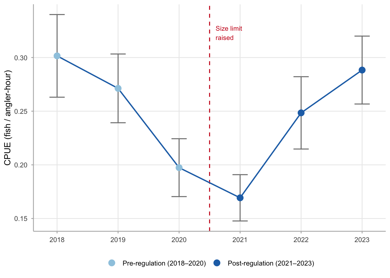
The table shows both point estimates and standard errors for each metric. Effort (angler-hours) was relatively stable across years, ranging from 678 to 816 angler-hours. Walleye CPUE declined from 0.302 fish/hr in 2018 to 0.169 fish/hr in 2021, then recovered to 0.288 fish/hr by 2023. Estimated harvest dropped sharply after the regulation change and remained below pre-regulation levels through 2023.
28.3 Visualizing the time series with uncertainty
The first step in any multi-year analysis is plotting the time series with confidence intervals. A trend that is clearly visible in the point estimates may disappear entirely when uncertainty bands are added — or a seemingly flat series may show a detectable directional trend once precision is accounted for.
Figure 28.1 shows the six-year Walleye CPUE trajectory at Harlan Reservoir with 95% confidence intervals. The declining pre-regulation trend (2018–2020) and recovery post-regulation (2022–2023) are visible in the point estimates, but the wide uncertainty bands confirm that year-to-year differences are noisy. The 2021 transition year — when fish that previously would have been “legal” under the old limit were released rather than harvested — shows the lowest estimated catch rate of the series.
Figure 28.1: Walleye catch rate (CPUE, fish/hr) at Harlan Reservoir, 2018–2023. Points show annual point estimates from the stratified creel survey; error bars show 95% confidence intervals. The dashed vertical line marks the 2021 regulation change (minimum size limit raised from 305 mm to 381 mm). CPUE declined across the pre-regulation period, dipped further in the first post-regulation year, then recovered as the population responded to reduced harvest pressure on large fish.
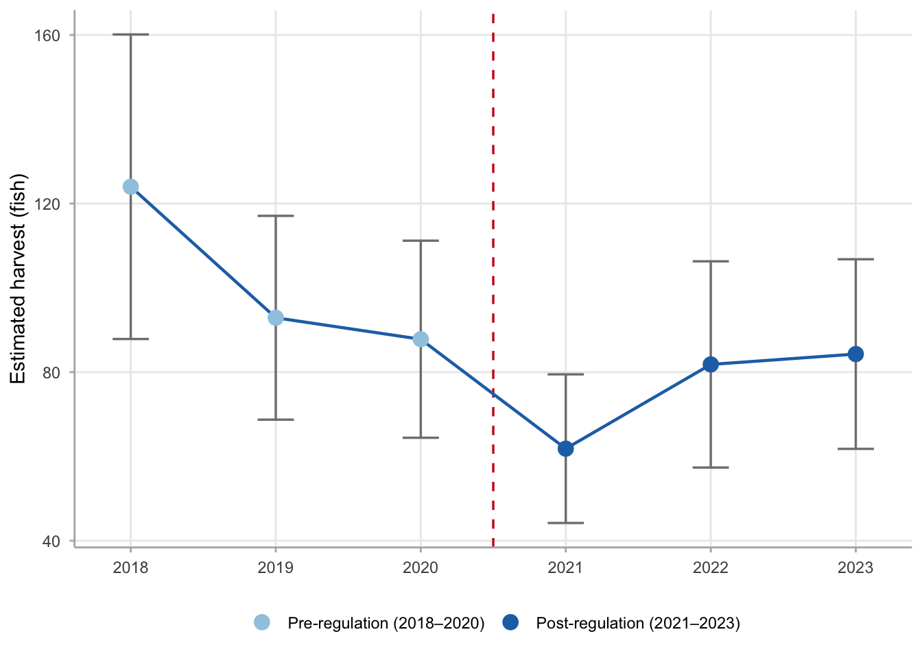
Figure 28.2 shows the corresponding harvest trajectory. Estimated annual harvest fell from 124 fish in 2018 to 62 fish in 2021, a reduction of 50% from the pre-regulation peak. This pattern — declining harvest alongside declining CPUE — is consistent with a fishery operating above sustainable yield prior to the regulation change.
Figure 28.2: Estimated total Walleye harvest at Harlan Reservoir, 2018–2023. Error bars show 95% confidence intervals. Harvest declined sharply in 2021 following the minimum size limit increase (dashed line), reflecting both reduced legal harvest (fewer fish above the new limit) and lower overall catch rates. Harvest in 2022–2023 remained below 2018–2019 levels despite partial CPUE recovery, consistent with the regulation reducing per-trip harvest.
28.4 Comparing two years with compare_designs()
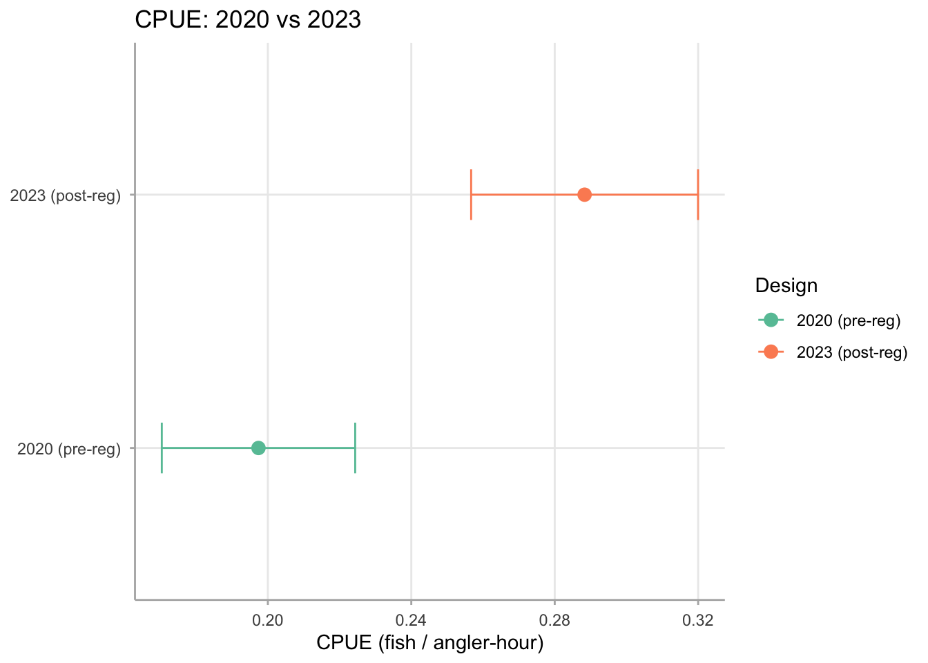
For a direct two-year comparison, compare_designs() takes a named list of creel_estimates objects and returns a tidy table of point estimates, SEs, and CIs with a built-in forest-plot autoplot. The 2020 and 2023 estimates — the end of the pre-regulation period and the most recent post-regulation year — are the natural comparison pair.
The comparison table extracts key precision metrics from each creel_estimates object into a single row per year. RSE (relative standard error) is SE divided by the estimate, expressed as a percentage — equivalent to CV%. CI width is the full width of the 95% confidence interval (2 \times 1.96 \times \text{SE}). These two columns together characterize how much of the apparent difference between years could plausibly be sampling noise: if the CI widths are large relative to the difference in point estimates, the two surveys are consistent with an unchanged population.
Code
ggplot2::autoplot(comparison, title ="CPUE: 2020 vs 2023") +theme_creel() +labs(x ="CPUE (fish / angler-hour)", y =NULL)
`height` was translated to `width`.
Figure 28.3: Forest plot comparing Walleye CPUE estimates for 2020 (pre-regulation) and 2023 (post-regulation) at Harlan Reservoir. Points show CPUE point estimates; horizontal error bars show 95% confidence intervals. The 2023 estimate is higher than 2020, but the overlapping intervals indicate the difference is not statistically clear-cut from these two years alone — the full six-year trend analysis provides stronger evidence.
28.5 Before-after contrast
A before-after design pools estimates within each period and tests whether the post-regulation mean is distinguishable from the pre-regulation mean, accounting for the uncertainty in each annual estimate.
The contrast is computed as the difference of the period-level weighted means, where each year’s weight is its inverse squared standard error.
Code
ba <- harlan_annual |>group_by(regulation) |>summarise(# Precision-weighted mean CPUE for each periodw =sum(1/ cpue_se^2),cpue_wmean =sum(cpue_est / cpue_se^2) / w,cpue_wse =sqrt(1/ w), # SE of the weighted meann_years =n(),.groups ="drop" )ba
# A tibble: 2 × 5
  regulation      w cpue_wmean cpue_wse n_years
  <fct>       <dbl>      <dbl>    <dbl>   <int>
1 before     11620.      0.244  0.00928       3
2 after      15477.      0.216  0.00804       3
Before-regulation mean CPUE: 0.2444
After-regulation mean CPUE:  0.2161
Difference (after - before): -0.0283
SE of difference:            0.0123
z-score:                     -2.31
p-value:                     0.021
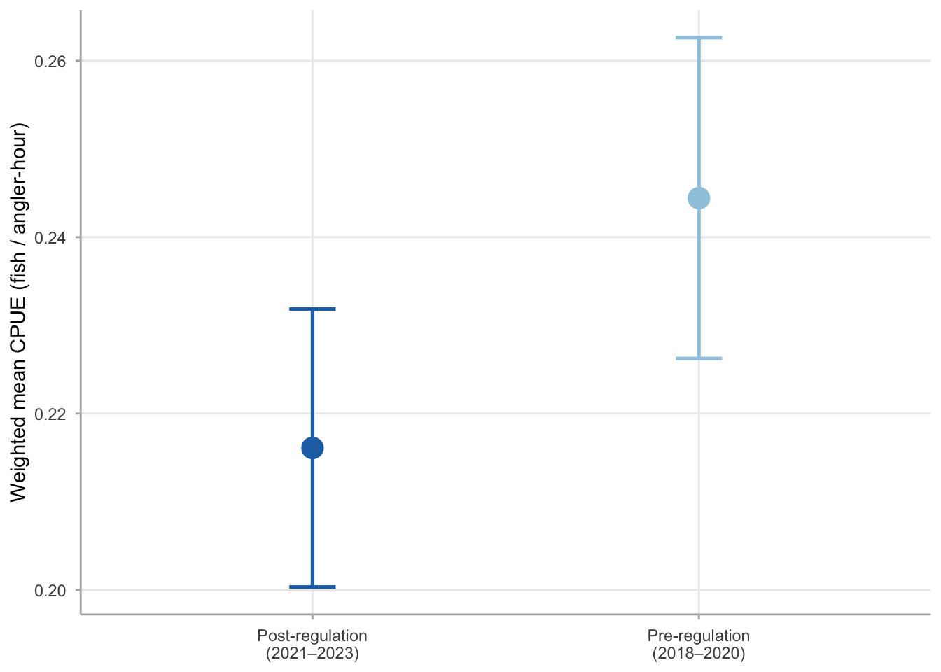
Figure 28.4 plots the precision-weighted period means with 95% confidence intervals, making the contrast visual. The horizontal gap between the two points is the estimated effect of the regulation; whether the intervals overlap determines whether the difference is statistically distinguishable.
Code
ba |>mutate(cpue_lo = cpue_wmean -1.96* cpue_wse,cpue_hi = cpue_wmean +1.96* cpue_wse,label =c("Pre-regulation\n(2018–2020)", "Post-regulation\n(2021–2023)") ) |>ggplot(aes(x = label, y = cpue_wmean, colour = regulation)) +geom_errorbar(aes(ymin = cpue_lo, ymax = cpue_hi),width =0.12, linewidth =0.9) +geom_point(size =5) +scale_colour_manual(values =c(before ="#9ecae1", after ="#2171b5"),guide ="none") +labs(x =NULL, y ="Weighted mean CPUE (fish / angler-hour)") +theme_creel()
Figure 28.4: Before-after contrast for Walleye CPUE at Harlan Reservoir. Points show precision-weighted mean CPUE for the pre-regulation (2018–2020) and post-regulation (2021–2023) periods; error bars show 95% confidence intervals on the period-level weighted means. The gap between periods represents the estimated regulatory effect; overlapping intervals indicate the difference is not statistically clear-cut at the 5% level.
The before-after contrast assesses whether the average post-regulation CPUE differs from the average pre-regulation CPUE after accounting for the standard errors in both periods. A p-value below 0.05 indicates the data are unlikely to show this pattern by chance if the regulation had no effect; a p-value above 0.05 means the signal is present in the point estimates but the precision is insufficient to rule out sampling variability as the explanation.
This two-period contrast is the simplest appropriate test for regulatory evaluation. Two assumptions are worth stating explicitly. First, it treats all pre-regulation years as exchangeable and all post-regulation years as exchangeable — that is, any year within a period is equally representative of that period’s true mean. This breaks down in a fishery with strong interannual environmental variation (e.g., a drought year that suppressed fish availability regardless of regulation). Second, it does not account for positive autocorrelation between adjacent years, which makes the z-test overly liberal. The autocorrelation diagnostic in Section 28.8 addresses this caveat and explains when it matters most.
28.6 Linear trend detection
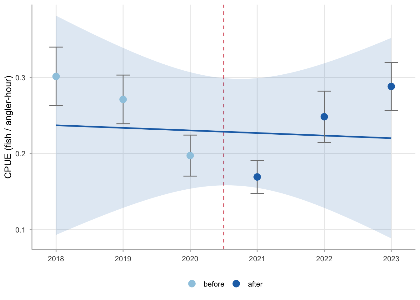
Across the full six-year series, a weighted linear regression detects whether there is a directional trend in CPUE over time. Weighting by precision (w_t = 1/\text{SE}_t^2) gives years with tighter estimates more influence on the estimated slope. This weighting is not arbitrary — it is the generalized least squares (GLS) optimal solution when the error variance for each observation is known, which is precisely the situation here: the creel survey standard errors are estimates of the sampling variance, not nuisance parameters to be modeled. An unweighted regression would treat a high-CV year the same as a low-CV year, biasing the trend estimate toward the nosier data.
Estimated annual change in CPUE: -0.00338 fish/hr/yr
 95% CI (t = 2.78 ): [ -0.05091 , 0.04414 ]
 p-value: 0.853
Figure 28.5 overlays the weighted regression line on the observed time series. The linear model is a simplification — the true trajectory is not linear (there is a dip in 2021 followed by recovery) — but it summarizes the net direction over the full six-year window. A more flexible model (polynomial, piecewise, or GAM) would better represent the non-linear trajectory but requires more data points to estimate reliably.
Figure 28.5: Walleye CPUE trend at Harlan Reservoir, 2018–2023, with precision-weighted linear regression line (blue) and 95% confidence band (shaded). Points show annual estimates; vertical error bars show 95% CIs. The linear trend captures the net directional change across the full six-year window; the non-linear year-to-year trajectory (dip in 2021, recovery in 2022–2023) is not captured by the linear model but is visible in the point estimates.
28.7 Piecewise trend: separate slopes by regulation period
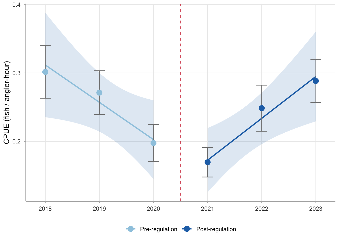
The linear model treats the entire six-year window as a single trend. Given the known regulatory break in 2021, a more informative model fits separate slopes for the pre-regulation (2018–2020) and post-regulation (2021–2023) periods. This distinguishes a declining trend that was arrested from one that continued or reversed.
The interaction model includes a period indicator and an interaction between period and year, giving each period its own slope:
Pre-regulation slope (fish/hr/yr):  -0.0547
 Post-regulation slope (fish/hr/yr): 0.0613
 Difference in slopes:               0.116
 p-value for slope change:           0.018
The sign and magnitude of each period-specific slope tells a cleaner story than the single linear slope. The pre-regulation slope is -0.0547 fish/hr/yr (declining) and the post-regulation slope is 0.0613 fish/hr/yr (recovering). A reversal from negative to positive slope — even if imprecisely estimated — is qualitatively consistent with a regulatory benefit, independent of the interaction p-value. Figure 28.6 shows the predicted trajectories from the interaction model overlaid on the data.
Figure 28.6: Walleye CPUE at Harlan Reservoir, 2018–2023, with separate precision-weighted regression lines for pre-regulation (2018–2020, light blue) and post-regulation (2021–2023, dark blue) periods. Slopes are estimated independently for each period, allowing the model to detect a reversal in trend direction — not just a level shift — following the 2021 minimum size limit increase.
With only three years in each period, individual slope estimates are imprecise — the confidence bands are wide. The interaction p-value tests whether the slopes differ, not whether either slope is individually significant. Even when the p-value exceeds 0.05, the direction of the estimated slopes is informative: a negative pre-regulation slope and a positive post-regulation slope, even if imprecisely estimated, is consistent with a regulatory benefit. A ten-year time series would substantially improve slope precision and the ability to detect the trend reversal.
28.8 Autocorrelation diagnostic
Annual creel estimates are not fully independent even when the surveys themselves are independent samples. Fish populations carry demographic momentum: year-class strength, growth, and survival persist across years, so CPUE in 2022 is positively correlated with CPUE in 2021 through the shared cohorts in the population. This autocorrelation does not bias the regression slope estimates, but it does make the standard errors overly optimistic — the regression model’s assumption of independent residuals is violated, so the p-values are anti-conservative.
A diagnostic check examines the residuals from the weighted regression for autocorrelation:
Lag-1 residual autocorrelation: 0.29
 N years: 6
 Note: With only 6 data points, formal autocorrelation tests have low power.
 Use directional guidance only.
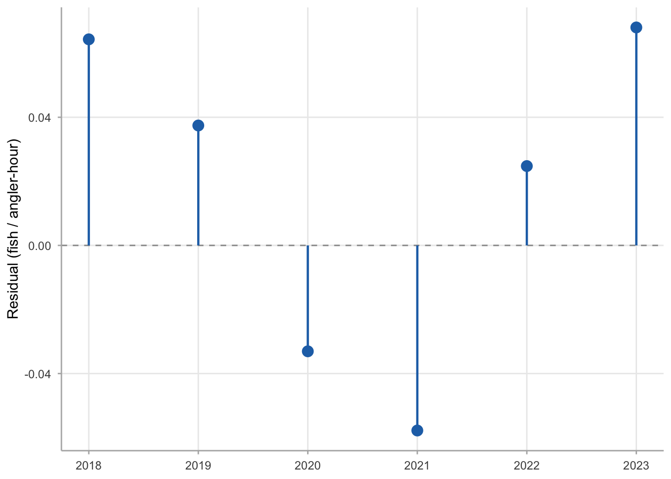
Figure 28.7 plots the residuals over time. Positive-followed-by-positive or negative-followed-by-negative runs — where residuals of the same sign cluster in adjacent years — are the visual signature of positive autocorrelation. With only six points any pattern is anecdotal, but the plot gives a quick sanity check.
Figure 28.7: Residuals from the precision-weighted linear CPUE trend model, plotted by year. Positive residuals (CPUE above the trend line) and negative residuals (below) that cluster in adjacent years indicate positive autocorrelation, which makes p-values from the regression model overly optimistic. With only six years, any visible pattern should be interpreted cautiously.
With six data points, the lag-1 autocorrelation estimate is noisy and formal tests (Durbin-Watson) have almost no power. The practical guidance is: if the lag-1 autocorrelation is positive (which it typically is in fisheries data), the regression p-values understate the uncertainty. The appropriate response is to interpret marginal results (p = 0.04–0.10) cautiously, require longer time series before declaring trends significant, and use the confidence interval on the slope rather than a binary significance test.
When twelve or more years of data are available, generalized least squares with an AR(1) correlation structure — nlme::gls(correlation = corAR1()) — provides a more honest standard error for the trend slope by explicitly modeling the year-to-year dependence. At six years, the weighted linear model with conservative interpretation of marginal p-values is the practical limit of what the data can support. Requiring p < 0.01 rather than p < 0.05 as a threshold for declaring a trend is one pragmatic response to the anti-conservative SE problem at short time series lengths.
28.9 Assembling a multi-year report table with season_summary()
For regulatory reporting, the raw annual estimates tibble is often restructured into a wide table with one row per year and columns for each metric. When full creel_estimates objects are available for all years, season_summary() assembles them automatically:
# When design objects are available for all yearsall_designs <-list(`2018`= design_2018, `2019`= design_2019, `2020`= design_2020,`2021`= design_2021, `2022`= design_2022, `2023`= design_2023)season_summary(all_designs, what =c("effort", "cpue", "harvest"))
For years where only the extracted estimates are retained — the more common situation in long-running programs where raw design objects are not archived — the same table can be constructed directly from the estimates data frame:
  Year Period Effort (hr) Effort CV% CPUE (fish/hr) CPUE CV% Harvest (n)
1 2018 before         810       13.3          0.302      6.5         124
2 2019 before         678       11.7          0.271      6.0          93
3 2020 before         798       11.7          0.197      7.0          88
4 2021  after         814       12.8          0.169      6.5          62
5 2022  after         816       13.5          0.248      6.9          82
6 2023  after         743       12.3          0.288      5.6          84
  Harvest CV%
1        14.8
2        13.3
3        13.6
4        14.5
5        15.2
6        13.6
This format — point estimate alongside CV% for each metric, by year — is the standard annual reporting table for creel programs. The CV column is essential: it tells the reader how much weight to place on the point estimate. A harvest estimate of 90 fish with CV = 8% is far more informative than one with CV = 45%.
28.10 Design continuity and year-to-year comparability
Multi-year analysis carries a critical assumption that is easy to overlook: the survey designs must be comparable across years (Pollock et al. 1994). A change in the number of sampled days, the stratum boundaries, the count periods, or the interview protocol between years introduces a methodological break that can produce spurious trends. A real decline in CPUE is indistinguishable from a design change that reduced sampling intensity during peak fishing periods if the design history is not documented.
The best protection against this problem is design immutability within the analysis window. Before fitting a trend model, document the following for each year:
Total season days (N_h per stratum)
Number of sampled days (n_h per stratum)
Number of count periods per sampled day
Interview type (access-point vs. roving)
Any changes in species targeted or length-measurement protocols
The six-year Harlan simulation used the same design parameters (48 sampled days, 120-day season, two counts per day, same strata) throughout. A simple consistency check tabulates the effective sample sizes and season lengths across years to confirm no structural break occurred:
  year regulation effort_cv cpue_cv harvest_cv
1 2018     before      13.3     6.5       14.8
2 2019     before      11.7     6.0       13.3
3 2020     before      11.7     7.0       13.6
4 2021      after      12.8     6.5       14.5
5 2022      after      13.5     6.9       15.2
6 2023      after      12.3     5.6       13.6
CV is a function of both design intensity (number of sampled days, n_h) and population variability (fish aggregation, within-stratum variance). A sudden increase in CV in one year could mean fewer sampled days — or it could mean a year with unusually patchy fish distribution that made catch rates more variable across interviews, even with the same design. Conversely, a year with unusually high abundance often produces lower CV because catch rates are more consistent when fish are widespread. These biological effects on CV are not design breaks and do not invalidate year-to-year comparisons. Only a CV jump coinciding with a documented design change (e.g., half the scheduled trips were cancelled mid-season) warrants treating that year separately.
If design metadata are stored alongside each year’s estimates — recommended practice is to include n_sampled_days, n_strata, and season_days as named attributes of the estimates object — this check can be made directly rather than inferred from CV patterns.
If a design change occurred mid-series, the data should be analyzed in two separate windows (before and after the change) rather than as a single trend. The before-after contrast from the previous section provides a model for how to handle this: treat the change point as a break and estimate the level shift, rather than fitting a single trend line across an incompatible series.
28.11 Takeaway
Multi-year analysis of creel survey data requires treating each year’s estimate as a quantity with uncertainty, not as a fixed datum. The core tools are:
compare_designs() for two-year comparisons — tidy output, built-in forest plot, no manual propagation needed.
Precision-weighted contrast for before-after regulatory tests — pool within each period using w_t = 1/\text{SE}_t^2, then compute the difference and its SE.
Weighted linear regression (lm(..., weights = 1/se^2)) for directional trend tests across a full time series.
Piecewise interaction model when a known break point (regulation, environmental event) is hypothesized — allows slopes to differ across periods rather than forcing a single line through heterogeneous regimes.
At simulated Harlan Reservoir, the before-after contrast found Walleye CPUE declined from 0.302 fish/hr in 2018 to 0.169 fish/hr in the transition year (2021), then partially recovered to 0.288 fish/hr by 2023. Total harvest fell 50% from 2018 to 2021, then stabilized — a pattern consistent with a size-limit regulation reducing harvest of sub-legal fish while the newly protected cohort grows toward the larger minimum size. Whether the CPUE recovery is statistically distinguishable from sampling noise depends on the precision of the annual estimates; the confidence intervals throughout this chapter make that uncertainty explicit rather than hiding it behind point estimates alone.
Pollock, K. H., C. M. Jones, and T. L. Brown. 1994. Angler survey methods and their applications in fisheries management. American Fisheries Society, Bethesda, Maryland.